流来！实时流体模拟的N种方法

本文汇总了常见的可以用到实时应用中的流体模拟技术。

本文中提到的所有算法都会附带单文件，直接可以运行的python代码。读者可以挑选喜欢的demo, 喂给agent放到游戏引擎中复现。

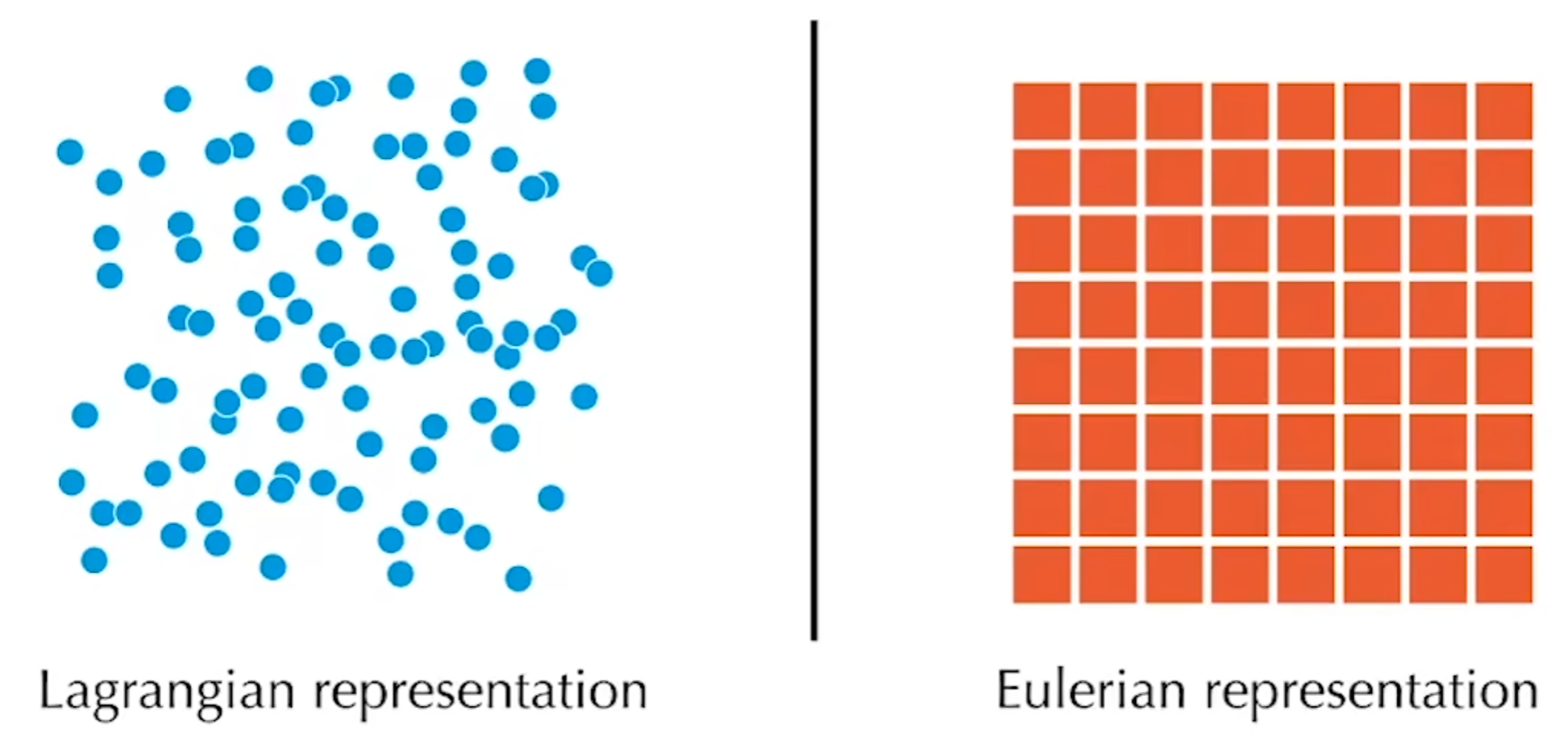
1. N-S方程速成

在介绍N-S方程之前，我们先介绍一下物理模拟的两大流派——拉格朗日视角和欧拉视角。（从Games201偷来的图）

简单来说，拉格朗日视角将流体看成大量携带质量的粒子，其模拟各个粒子在世界空间中的移动来实现整个流体的模拟。一个比较直观的现实例子是海洋球池，大量海洋球的运动从远处看上去像是水在流动。

拉格朗日视角下的N-S方程如公式(1.1)所示。

其中 为速度， 为密度， 为外力（的加速度）, 为粘性系数， 为物质导数，你暂时可以将其想成就是普通的全微分（我们将在和欧拉视角对比的时候详细介绍它！）。

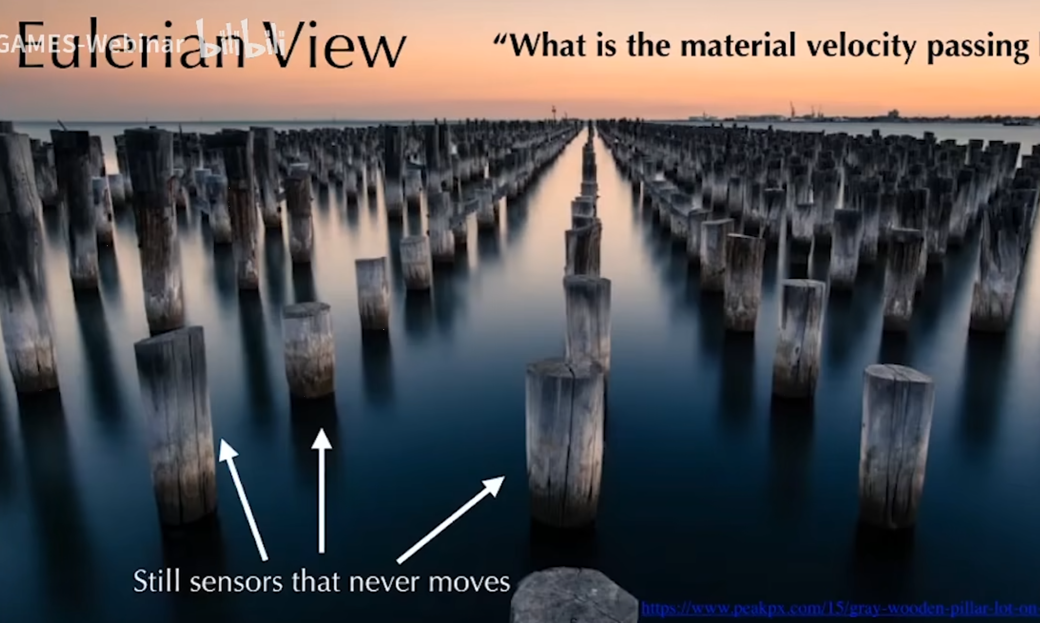
而欧拉视角则是会在流体内部插入固定的木桩（固定网格），每个木桩记录流体的变化并推算未来流体的走势。（又是从Games201偷来的图）

在欧拉视角下的N-S方程如公式(1.2)所示

公式(1.1)左边奇怪的物质导数消失了！取而代之的是更加奇怪的 这项。而这两项是建立起拉格朗日视角和欧拉视角之间联系的重要桥梁。

在拉格朗日视角下等价于单个粒子的加速度，因为 本质上就是速度对时间的全微分。对于速度场 有公式(1.3)

将 带入方程(1.1)左边后，方程就变成了欧拉视角下的N-S方程(1.2)，而 这项也就是我们常说的平流项(advection) 。

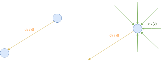
想要直观理解平流项从何而来，就要理解拉格朗日视角和欧拉视角的核心区别：观察者的位置不同。如下图所示。左边展示了在拉格朗日视角下，观察者会随着水粒子的运动移动，其时时刻刻观察的是同一个水粒子，因此他观察到的是同一个水粒子的速度随着时间变化。右边展示了在欧拉视角，观察者的位置不变，他不但能观察到观察点的水粒子速度的变化(黄色部分) ，还能观察到水从该点四周流入了 ，这些水流入该点对速度的总贡献为 （绿色部分）。

现在看向方程(1.1) (1.2) 的右边， 很好理解就是水粒子的外力（重力，交互产生的应力等）。 是粘性项（也被叫做扩散项），其定义了这个流体到底有多粘。其中 是在将粒子与四周的粒子的速度做平均，而 定义了这种平均效应的权重。 则是压力项，就是我们初中物理中学到的水体压强（在笔者受到的义务教育中是初中）。特别注意，是标量，液体在固定位置对各个方向的压强是相同的。这些概念很重要，我们后面将直接用这些名字称呼，在这里我们做一个小表格记录。

名称	公式
平流
外力
扩散
压力

整个方程比较特殊的就是压力项 ，一般需要通过别的条件间接推算出来。比如在做液体模拟的时候会假设液体是不可压缩的 （气体这方面约束应该会弱很多），此时，压力项通过联立不可压缩条件求解。

另一个观察N-S方程的有趣视角是，N-S方程可以看成特殊的牛顿第二定律。 实际上就是流体质点的加速度， 是外力；扩散项 就是流体质点的摩擦力；而压力项()由不可压缩条件 推导出来，其可视作一个粒子移动到一个地方挤压另一个粒子产生的效应，也就是流体质点之间碰撞产生的冲量。可以看到，N-S方程中的各项可以和刚体模拟中的各个概念一一对应上，确实可以说就是建立在流体微团上的牛顿第二定律。

前一阵子OpenAI公布解决的千禧年难题，其实就是找到了N-S方程的爆破解。这意味着用牛顿第二定律建模的N-S方程描述的流体会在一定条件下速度达到无穷，这在现实中是不成立的，也就是说N-S方程的建模不是完美的（牛顿描述的世界，并非完美），现实中一定存在其它要素会影响流体的运动。而网上一堆营销号铺天盖地的宣传N-S方程已经被解决，大肆宣扬AI焦虑的就显得很奇异搞笑了。

2. 拉格朗日视角

2.1 Smooth Particle Hydrodynamics

对于拉格朗日视角，有个重要问题需要解决：粒子都是离散且分布不规则的，如何计算密度，压力等连续场函数以及其梯度，散度？

SPH通过将粒子视作携带了物理量的核函数，对核函数加权求和重建连续场来解决这个问题。

核函数如上图所示，其中间高四周低，每个点对应粒子的物理量在该点对应的权重。想要计算一个物理量 只需要对周围的粒子加权求和：

其中 为粒子 的体积， 为粒子 的位置， 为核函数的半径， 为核函数权重。

例如对于密度有

在SPH中一般选立方样条曲线作为核函数。

SPH的梯度求解也十分简单，由于公式(2.1.1)中 这些粒子属性不会随着位置的变化而变化，因此对 求梯度就是在对核函数求梯度：

下面我将介绍SPH方法中最原始的一个变种WCSPH：

回到拉格朗日视角下的N-S方程

对于方程中的密度 ，可以直接用公式(2.1.2)计算。

对于压强 , WCSPH使用了弱可压缩(Weak Compress)假设，这也是WCSPH方法中WC 两个字母的来源。具体来说，我们不再要求求解后严格满足 ，而是用一个启发式函数估算每个点的压强。如公式(2.1.6)所示。

其中 是可调节参数， 是rest状态下的密度， 是当前粒子的密度。

这个公式可以在 时，产生压强，接着让粒子沿着压强梯度方向推开，从而让密度恢复到 ，实现不可压缩。

在实战中，可以先用公式(2.1.6)算出各个粒子的压强，接着用公式(2.1.4)算出对应的梯度，带入到压力项中，实现压力加速度的计算。

最后，扩散项可以有多种求解方法，这里给出其中两种。

1. 计算粒子周围的平均速度，接着和当前速度加权求和
2. 直接计算 ，其中 为当前系统的维度。带入到公式(2.1.5)中和计算。

公式(2.1.5)中的压力梯度 以及公式扩散项项 都涉及遍历每个粒子 半径范围内的粒子。用直接遍历将会是 的复杂度。为了加速，我们需要neighbor grid数据结构加速查询。Neighbor grid本质上就是记录了与每个单位空间格相交粒子的Hashtable。粒子在模拟时只需遍历其所处Hash grid格子内记录的所有粒子即可，大大降低了相交检测的粒子数量。

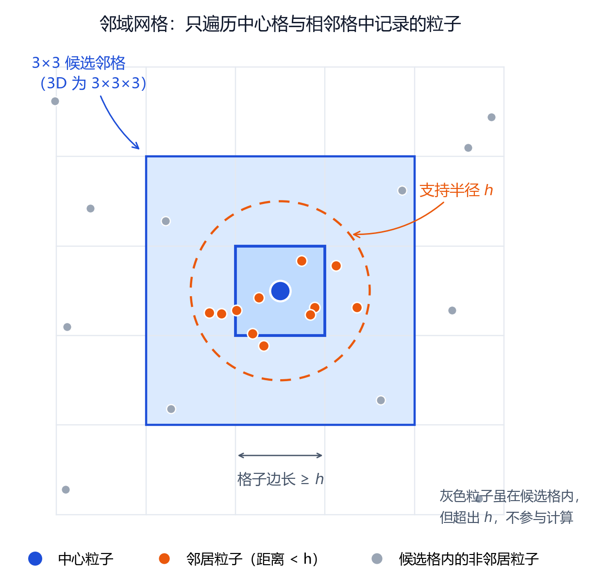
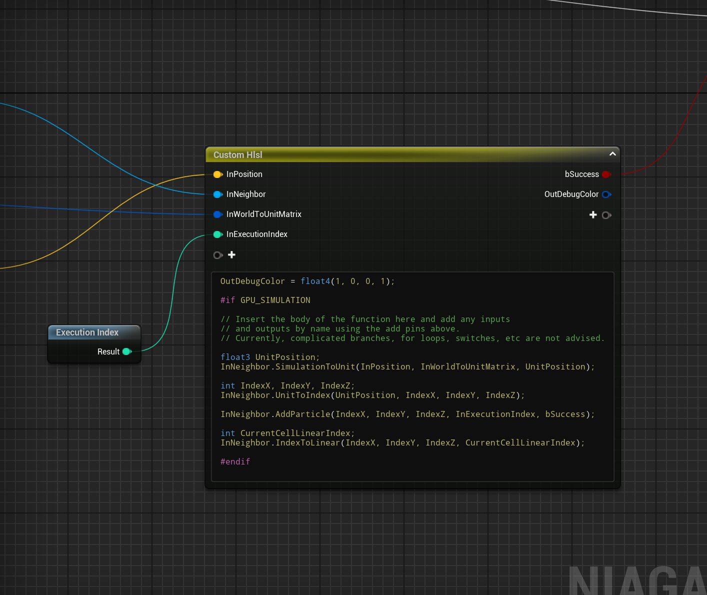
对于想要亲手实现一遍Neighbor Grid的同学，可以考虑参考UE5 Niagara中的实现。具体来说，一个Neighbor Grid是一个NxNxN的数组，每个格子内有E+1个元素。其中一个元素记录当前格子中相交的粒子数量，其余E个元素存与当前Neighbor Grid相交的粒子的索引。

运行时需要提供两个功能，更新网格和查询网格。

更新时逐个遍历粒子，计算每个粒子相交的格点，将该粒子添加到该格点相交元素队列中。在GPU或多线程实现中，你可能需要注意原子操作：

for(int ParticleIndex : PartialCount)
{
	int3 NeighborGridIndex = Intersect(ParticlePosition[ParticleIndex]);
    // AtomicAdd对指定内存值做加法，返回加法前的旧值，这个旧值就是分配给新元素的地址
    int NeighborGridInteralIndex = AtomicAdd(NeighborGrid[NeighborGridIndex].Count, 1);
    // Count可能会超过上限E, 这种情况分配的位置是不合法的，我们直接舍弃掉
    if(NeighborGridInteralIndex < E)
    {
    	   NeighborGrid[NeighborGridIndex].Arr[NeighborGridInteralIndex] = ParticleIndex;
    }
}

随后查询时，我们只需要遍历相交格点内的每一个元素即可。

for(int ParticleIndex : PartialCount)
{
	int3 NeighborGridIndex = Intersect(ParticlePosition[ParticleIndex]);
	// 遍历所有邻居
	for(int NeighborParticleInteralIndex = 0; NeighborParticleInteralIndex < NeighborGrid[NeighborGridIndex].Count; NeighborParticleInteralIndex++)
	{
		// 获取邻居索引
		int NeighborParticleIndex = NeighborGrid[NeighborGridIndex].Arr[ParticleNeighborInteralIndex];
		...
	}
}

整个模拟过程的伪代码类似：

def simulate():
	build_neighbor_grid()# 构建neighbor grid
    compute_density() # 公式(2.1.2)
	for particle in particles:
        pressure = compute_pressure_divergence(particle) # 公式(2.1.6)
        vis = compute_viscocity(particle) #前面说的几种计算粘性项方法中的任意一种
        particle.velocity = solve_velocity(pressure, vis) #公式 (2.1.5)

最后给出python实现

（感谢taichiCourse01/taichi_sph 开源）

"""Standalone 2D WCSPH simulation (single-file).

Self-contained version of the WCSPH demo. Dependencies: taichi, numpy.
Run with: python wcsph_standalone.py
代码改自 https://github.com/taichiCourse01/taichi_sph
"""

import taichi as ti
import numpy as np
from functools import reduce


@ti.data_oriented
class ParticleSystem:
    def __init__(self, res):
        self.res = res
        self.dim = len(res)
        assert self.dim > 1
        self.screen_to_world_ratio = 50
        self.bound = np.array(res) / self.screen_to_world_ratio
        # Material
        self.material_boundary = 0
        self.material_fluid = 1

        self.particle_radius = 0.05  # particle radius
        self.particle_diameter = 2 * self.particle_radius
        self.support_radius = self.particle_radius * 4.0  # support radius
        self.m_V = 0.8 * self.particle_diameter ** self.dim
        self.particle_max_num = 2 ** 15
        self.particle_max_num_per_cell = 100
        self.particle_max_num_neighbor = 100
        self.particle_num = ti.field(int, shape=())

        # Grid related properties
        self.grid_size = self.support_radius
        self.grid_num = np.ceil(np.array(res) / self.grid_size).astype(int)
        self.grid_particles_num = ti.field(int)
        self.grid_particles = ti.field(int)
        self.padding = self.grid_size

        # Particle related properties
        self.x = ti.Vector.field(self.dim, dtype=float)
        self.v = ti.Vector.field(self.dim, dtype=float)

        self.density = ti.field(dtype=float)
        self.pressure = ti.field(dtype=float)
        self.material = ti.field(dtype=int)
        self.color = ti.field(dtype=int)
        self.particle_neighbors = ti.field(int)
        self.particle_neighbors_num = ti.field(int)

        self.particles_node = ti.root.dense(ti.i, self.particle_max_num)
        self.particles_node.place(self.x, self.v, self.density, self.pressure, self.material, self.color)
        self.particles_node.place(self.particle_neighbors_num)
        self.particle_node = self.particles_node.dense(ti.j, self.particle_max_num_neighbor)
        self.particle_node.place(self.particle_neighbors)

        index = ti.ij if self.dim == 2 else ti.ijk
        grid_node = ti.root.dense(index, self.grid_num)
        grid_node.place(self.grid_particles_num)

        cell_index = ti.k if self.dim == 2 else ti.l
        cell_node = grid_node.dense(cell_index, self.particle_max_num_per_cell)
        cell_node.place(self.grid_particles)

    @ti.func
    def add_particle(self, p, x, v, density, pressure, material, color):
        self.x[p] = x
        self.v[p] = v
        self.density[p] = density
        self.pressure[p] = pressure
        self.material[p] = material
        self.color[p] = color
        self.init_particle_extra(p, x, v)

    @ti.kernel
    def add_particles(self, new_particles_num: int,
                      new_particles_positions: ti.types.ndarray(),
                      new_particles_velocity: ti.types.ndarray(),
                      new_particle_density: ti.types.ndarray(),
                      new_particle_pressure: ti.types.ndarray(),
                      new_particles_material: ti.types.ndarray(),
                      new_particles_color: ti.types.ndarray()):
        for p in range(self.particle_num[None], self.particle_num[None] + new_particles_num):
            v = ti.Vector.zero(float, self.dim)
            x = ti.Vector.zero(float, self.dim)

            for d in ti.static(range(self.dim)):
                v[d] = new_particles_velocity[p - self.particle_num[None], d]
                x[d] = new_particles_positions[p - self.particle_num[None], d]
            self.add_particle(p, x, v,
                              new_particle_density[p - self.particle_num[None]],
                              new_particle_pressure[p - self.particle_num[None]],
                              new_particles_material[p - self.particle_num[None]],
                              new_particles_color[p - self.particle_num[None]])
        self.particle_num[None] += new_particles_num

    @ti.func
    def pos_to_index(self, pos):
        return (pos / self.grid_size).cast(int)

    @ti.func
    def is_valid_cell(self, cell):
        # Check whether the cell is in the grid
        flag = True
        for d in ti.static(range(self.dim)):
            flag = flag and (0 <= cell[d] < self.grid_num[d])
        return flag

    @ti.func
    def search_position(self, p):
        # Position used to build the spatial grid and neighbor lists.
        # Subclasses (e.g. PBDParticleSystem) can override this to use pred_x.
        return self.x[p]

    @ti.func
    def init_particle_extra(self, p, x, v):
        # Hook for subclasses to initialize their own per-particle state.
        pass

    @ti.kernel
    def allocate_particles_to_grid(self):
        for p in range(self.particle_num[None]):
            cell = self.pos_to_index(self.search_position(p))
            offset = ti.atomic_add(self.grid_particles_num[cell], 1)
            self.grid_particles[cell, offset] = p

    @ti.kernel
    def search_neighbors(self):
        for p_i in range(self.particle_num[None]):
            # Skip boundary particles
            if self.material[p_i] == self.material_boundary:
                continue
            x_i = self.search_position(p_i)
            center_cell = self.pos_to_index(x_i)
            cnt = 0
            for offset in ti.grouped(ti.ndrange(*((-1, 2),) * self.dim)):
                if cnt >= self.particle_max_num_neighbor:
                    break
                cell = center_cell + offset
                if not self.is_valid_cell(cell):
                    break
                for j in range(self.grid_particles_num[cell]):
                    p_j = self.grid_particles[cell, j]
                    distance = (x_i - self.search_position(p_j)).norm()
                    if cnt < self.particle_max_num_neighbor and p_i != p_j and distance < self.support_radius:
                        self.particle_neighbors[p_i, cnt] = p_j
                        cnt += 1
            self.particle_neighbors_num[p_i] = cnt

    def initialize_particle_system(self):
        self.grid_particles_num.fill(0)
        self.particle_neighbors.fill(-1)
        self.allocate_particles_to_grid()
        self.search_neighbors()

    @ti.kernel
    def copy_to_numpy_nd(self, np_arr: ti.types.ndarray(), src_arr: ti.template()):
        for i in range(self.particle_num[None]):
            for j in ti.static(range(self.dim)):
                np_arr[i, j] = src_arr[i][j]

    @ti.kernel
    def copy_to_numpy(self, np_arr: ti.types.ndarray(), src_arr: ti.template()):
        for i in range(self.particle_num[None]):
            np_arr[i] = src_arr[i]

    def dump(self):
        np_x = np.ndarray((self.particle_num[None], self.dim), dtype=np.float32)
        self.copy_to_numpy_nd(np_x, self.x)

        np_v = np.ndarray((self.particle_num[None], self.dim), dtype=np.float32)
        self.copy_to_numpy_nd(np_v, self.v)

        np_material = np.ndarray((self.particle_num[None],), dtype=np.int32)
        self.copy_to_numpy(np_material, self.material)

        np_color = np.ndarray((self.particle_num[None],), dtype=np.int32)
        self.copy_to_numpy(np_color, self.color)

        return {
            'position': np_x,
            'velocity': np_v,
            'material': np_material,
            'color': np_color
        }

    def add_cube(self,
                 lower_corner,
                 cube_size,
                 material,
                 color=0xFFFFFF,
                 density=None,
                 pressure=None,
                 velocity=None):

        num_dim = []
        for i in range(self.dim):
            num_dim.append(
                np.arange(lower_corner[i], lower_corner[i] + cube_size[i],
                          self.particle_radius))
        num_new_particles = reduce(lambda x, y: x * y,
                                   [len(n) for n in num_dim])
        assert self.particle_num[
                   None] + num_new_particles <= self.particle_max_num

        new_positions = np.array(np.meshgrid(*num_dim,
                                             sparse=False,
                                             indexing='ij'),
                                 dtype=np.float32)
        new_positions = new_positions.reshape(-1,
                                              reduce(lambda x, y: x * y, list(new_positions.shape[1:]))).transpose()
        print("new position shape ", new_positions.shape)
        if velocity is None:
            velocity = np.full_like(new_positions, 0)
        else:
            velocity = np.array([velocity for _ in range(num_new_particles)], dtype=np.float32)

        material = np.full_like(np.zeros(num_new_particles), material)
        color = np.full_like(np.zeros(num_new_particles), color)
        density = np.full_like(np.zeros(num_new_particles), density if density is not None else 1000.)
        pressure = np.full_like(np.zeros(num_new_particles), pressure if pressure is not None else 0.)
        self.add_particles(num_new_particles, new_positions, velocity, density, pressure, material, color)


@ti.data_oriented
class SPHBase:
    def __init__(self, particle_system):
        self.ps = particle_system
        self.g = -9.80  # Gravity
        self.viscosity = 0.3  # viscosity
        self.density_0 = 1000.0  # reference density
        self.mass = self.ps.m_V * self.density_0
        self.dt = ti.field(float, shape=())
        self.dt[None] = 2e-4

    @ti.func
    def cubic_kernel(self, r_norm):
        res = ti.cast(0.0, ti.f32)
        h = self.ps.support_radius
        # value of cubic spline smoothing kernel
        k = 1.0
        if self.ps.dim == 1:
            k = 4 / 3
        elif self.ps.dim == 2:
            k = 40 / 7 / np.pi
        elif self.ps.dim == 3:
            k = 8 / np.pi
        k /= h ** self.ps.dim
        q = r_norm / h
        if q <= 1.0:
            if q <= 0.5:
                q2 = q * q
                q3 = q2 * q
                res = k * (6.0 * q3 - 6.0 * q2 + 1)
            else:
                res = k * 2 * ti.pow(1 - q, 3.0)
        return res

    @ti.func
    def cubic_kernel_derivative(self, r):
        h = self.ps.support_radius
        # derivative of cubic spline smoothing kernel
        k = 1.0
        if self.ps.dim == 1:
            k = 4 / 3
        elif self.ps.dim == 2:
            k = 40 / 7 / np.pi
        elif self.ps.dim == 3:
            k = 8 / np.pi
        k = 6. * k / h ** self.ps.dim
        r_norm = r.norm()
        q = r_norm / h
        res = ti.Vector([0.0 for _ in range(self.ps.dim)])
        if r_norm > 1e-5 and q <= 1.0:
            grad_q = r / (r_norm * h)
            if q <= 0.5:
                res = k * q * (3.0 * q - 2.0) * grad_q
            else:
                factor = 1.0 - q
                res = k * (-factor * factor) * grad_q
        return res

    @ti.func
    def viscosity_force(self, p_i, p_j, r):
        # Compute the viscosity force contribution
        v_xy = (self.ps.v[p_i] -
                self.ps.v[p_j]).dot(r)
        res = 2 * (self.ps.dim + 2) * self.viscosity * (self.mass / (self.ps.density[p_j])) * v_xy / (
            r.norm()**2 + 0.01 * self.ps.support_radius**2) * self.cubic_kernel_derivative(
                r)
        return res

    @ti.func
    def pressure_force(self, p_i, p_j, r):
        # Compute the pressure force contribution, Symmetric Formula
        res = -self.density_0 * self.ps.m_V * (self.ps.pressure[p_i] / self.ps.density[p_i] ** 2
              + self.ps.pressure[p_j] / self.ps.density[p_j] ** 2) \
              * self.cubic_kernel_derivative(r)
        return res

    def substep(self):
        pass

    @ti.func
    def simulate_collisions(self, p_i, vec, d):
        # Collision factor, assume roughly (1-c_f)*velocity loss after collision
        c_f = 0.3
        self.ps.x[p_i] += vec * d
        self.ps.v[p_i] -= (
            1.0 + c_f) * self.ps.v[p_i].dot(vec) * vec

    @ti.kernel
    def enforce_boundary(self):
        for p_i in range(self.ps.particle_num[None]):
            if self.ps.dim == 2:
                if self.ps.material[p_i] == self.ps.material_fluid:
                    pos = self.ps.x[p_i]
                    if pos[0] < self.ps.padding:
                        self.simulate_collisions(
                            p_i, ti.Vector([1.0, 0.0]),
                            self.ps.padding - pos[0])
                    if pos[0] > self.ps.bound[0] - self.ps.padding:
                        self.simulate_collisions(
                            p_i, ti.Vector([-1.0, 0.0]),
                            pos[0] - (self.ps.bound[0] - self.ps.padding))
                    if pos[1] > self.ps.bound[1] - self.ps.padding:
                        self.simulate_collisions(
                            p_i, ti.Vector([0.0, -1.0]),
                            pos[1] - (self.ps.bound[1] - self.ps.padding))
                    if pos[1] < self.ps.padding:
                        self.simulate_collisions(
                            p_i, ti.Vector([0.0, 1.0]),
                           self.ps.padding - pos[1])

    def step(self):
        self.ps.initialize_particle_system()
        self.substep()
        self.enforce_boundary()


class WCSPHSolver(SPHBase):
    def __init__(self, particle_system, dt = 4e-5):
        super().__init__(particle_system)
        # Pressure state function parameters(WCSPH)
        self.exponent = 7.0
        self.stiffness = 50.0
        self.dt[None] = dt

        self.d_velocity = ti.Vector.field(self.ps.dim, dtype=float)
        particle_node = ti.root.dense(ti.i, self.ps.particle_max_num)
        particle_node.place(self.d_velocity)

    @ti.kernel
    def compute_densities(self):
        for p_i in range(self.ps.particle_num[None]):
            x_i = self.ps.x[p_i]
            self.ps.density[p_i] = 0.0
            for j in range(self.ps.particle_neighbors_num[p_i]):
                p_j = self.ps.particle_neighbors[p_i, j]
                x_j = self.ps.x[p_j]
                self.ps.density[p_i] += self.ps.m_V * self.cubic_kernel((x_i - x_j).norm())
            self.ps.density[p_i] *= self.density_0

    @ti.kernel
    def compute_pressure_forces(self):
        for p_i in range(self.ps.particle_num[None]):
            self.ps.density[p_i] = ti.max(self.ps.density[p_i], self.density_0)
            self.ps.pressure[p_i] = self.stiffness * (ti.pow(self.ps.density[p_i] / self.density_0, self.exponent) - 1.0)
        for p_i in range(self.ps.particle_num[None]):
            if self.ps.material[p_i] != self.ps.material_fluid:
                continue
            x_i = self.ps.x[p_i]
            d_v = ti.Vector([0.0 for _ in range(self.ps.dim)])
            for j in range(self.ps.particle_neighbors_num[p_i]):
                p_j = self.ps.particle_neighbors[p_i, j]
                x_j = self.ps.x[p_j]
                # Compute Pressure force contribution
                d_v += self.pressure_force(p_i, p_j, x_i-x_j)
            self.d_velocity[p_i] += d_v

    @ti.kernel
    def compute_non_pressure_forces(self):
        for p_i in range(self.ps.particle_num[None]):
            if self.ps.material[p_i] != self.ps.material_fluid:
                continue
            x_i = self.ps.x[p_i]
            # Add body force
            d_v = ti.Vector([0.0 for _ in range(self.ps.dim)])
            d_v[self.ps.dim-1] = self.g
            for j in range(self.ps.particle_neighbors_num[p_i]):
                p_j = self.ps.particle_neighbors[p_i, j]
                x_j = self.ps.x[p_j]
                d_v += self.viscosity_force(p_i, p_j, x_i - x_j)
            self.d_velocity[p_i] = d_v

    @ti.kernel
    def advect(self):
        # Symplectic Euler
        for p_i in range(self.ps.particle_num[None]):
            if self.ps.material[p_i] == self.ps.material_fluid:
                self.ps.v[p_i] += self.dt[None] * self.d_velocity[p_i]
                self.ps.x[p_i] += self.dt[None] * self.ps.v[p_i]

    def substep(self):
        self.compute_densities()
        self.compute_non_pressure_forces()
        self.compute_pressure_forces()
        self.advect()

ti.init(arch=ti.gpu)

if __name__ == "__main__":
    ps = ParticleSystem((512, 512))
    solver = WCSPHSolver(ps, dt=1e-3)

    ps.add_cube(lower_corner=[6, 2],
                cube_size=[3.0, 5.0],
                velocity=[-5.0, -10.0],
                density=1000.0,
                color=0x956333,
                material=1)

    ps.add_cube(lower_corner=[3, 1],
                cube_size=[2.0, 6.0],
                velocity=[0.0, -20.0],
                density=1000.0,
                color=0x956333,
                material=1)

    ps.add_cube(lower_corner=[1, 3],
                cube_size=[1.9, 2.0],
                velocity=[5.0, -10.0],
                density=1000.0,
                color=0x956333,
                material=1)

    gui = ti.GUI(background_color=0xFFFFFF)
    iter = 0
    while gui.running:
        if iter == 1:
            iter = 0
            solver.step()
        iter += 1
        particle_info = ps.dump()
        gui.circles(particle_info['position'] * ps.screen_to_world_ratio / 512,
                    radius=ps.particle_radius / 1.5 * ps.screen_to_world_ratio,
                    color=0x956333)
        gui.show()

对于懒得跑代码的大忙人，这里放一下运行的结果。（连叫agent帮你装个python都不乐意吗，大忙人，你这个家伙…）

2.2 Position Based Fluid

说到物理模拟不得不提到我们物理模拟界的原神——PBD。而Position based fluids | ACM Transactions on Graphics 就将PBD和SPH缝在了一起，实现了更稳定的压力项求解。

在介绍PBD前首先需要介绍约束。

在物理系统中，一个约束 就是这个系统必须满足的条件。例如，有两个刚体相撞，则必须在接触点满足不重叠的约束。

在传统物理引擎中，一般都是通过求解 来计算两个刚体（粒子）之间的力，接着由力更新速度，最后由速度更新两个刚体（粒子）的位置。

而在PBD中，这个流程反了过来，系统先求解满足 的位置，接着由刚体（粒子）位置反过来推测两个刚体（粒子）的速度。

PBD中 为粒子位置 的函数，返回一个标量，代表当前状态距离满足约束还有多远。而系统必须满足 大于等于0或者等于0。

例如，对于两个刚体相撞， 可以表示为：

其中 为两个刚体的位置以及旋转， 为local space下两个刚体接触点的坐标， 为接触点的法线。

PBD的核心求解循环有以下几步：

1. 积分：计算

2. 碰撞检测：收集系统中的所有约束

3. 求解约束：多次迭代，每次迭代计算 ， 的值如公式(2.2.1),(2.2.2)所示。其中 为粒子质量的倒数。为了简洁这里不展开介绍公式的推导，有兴趣的可以看PBD原论文。
   

4. 反向更新速度：

有了PBD的基础接下来我们来介绍如何将PBD应用到SPH方法中。

还记得公式(1.4)中对NS方程的拆解吗，根据拆解可以将NS方程的求解分为：

def solve():
	solve_external_force()# 计算外力项 g
	solve_pressure()# 计算压力项p
	solve_viscosity()# 计算粘性项mu

其中最困难的就是solve_pressure 计算压力。

Position Based Fluid的解决方案是将压力项放到PBD框架下求解，具体来说，它给每个粒子都构建了一个等密度约束：

其中可以利用公式(2.1.2)计算。

对 求梯度有公式(2.2.4)

为了保证数值稳定，作者在分母上加了个微小量 保证数值稳定

由于SPH假定每个粒子的质量相同因此 被提出，后续该项会被分子中的 消去。

对于 ，要加上所有 的贡献：

推导到这里已经闭环了。把公式(2.2.4)→(2.2.5)→(2.2.6) 与本章开头的 PBD 求解循环对上，可以看到三条主线：公式(2.2.4) 给出 的两个分支——对角项（）是所有邻居核函数梯度之和，非对角项（）是单个邻居的核函数梯度取负；公式(2.2.5) 用”梯度的模长平方和”作分母，把残差 折算成拉格朗日乘子 ；公式(2.2.6) 再把所有约束（ 自己的 加上邻居们的 ）对粒子 的作用叠加起来，得到位移增量。之后

正好就是求解循环的第 3、4 步，压力项在 PBD 框架下的求解到此结束。

"""Standalone 2D PBD Fluid simulation (single-file).

Self-contained version of the PBD Fluid demo. Dependencies: taichi, numpy.
Run with: python pbd_standalone.py
"""

import taichi as ti
import numpy as np
from functools import reduce


@ti.data_oriented
class ParticleSystem:
    def __init__(self, res):
        self.res = res
        self.dim = len(res)
        assert self.dim > 1
        self.screen_to_world_ratio = 50
        self.bound = np.array(res) / self.screen_to_world_ratio
        # Material
        self.material_boundary = 0
        self.material_fluid = 1

        self.particle_radius = 0.05  # particle radius
        self.particle_diameter = 2 * self.particle_radius
        self.support_radius = self.particle_radius * 4.0  # support radius
        self.m_V = 0.8 * self.particle_diameter ** self.dim
        self.particle_max_num = 2 ** 15
        self.particle_max_num_per_cell = 100
        self.particle_max_num_neighbor = 100
        self.particle_num = ti.field(int, shape=())

        # Grid related properties
        self.grid_size = self.support_radius
        self.grid_num = np.ceil(np.array(res) / self.grid_size).astype(int)
        self.grid_particles_num = ti.field(int)
        self.grid_particles = ti.field(int)
        self.padding = self.grid_size

        # Particle related properties
        self.x = ti.Vector.field(self.dim, dtype=float)
        self.v = ti.Vector.field(self.dim, dtype=float)

        self.density = ti.field(dtype=float)
        self.pressure = ti.field(dtype=float)
        self.material = ti.field(dtype=int)
        self.color = ti.field(dtype=int)
        self.particle_neighbors = ti.field(int)
        self.particle_neighbors_num = ti.field(int)

        self.particles_node = ti.root.dense(ti.i, self.particle_max_num)
        self.particles_node.place(self.x, self.v, self.density, self.pressure, self.material, self.color)
        self.particles_node.place(self.particle_neighbors_num)
        self.particle_node = self.particles_node.dense(ti.j, self.particle_max_num_neighbor)
        self.particle_node.place(self.particle_neighbors)

        index = ti.ij if self.dim == 2 else ti.ijk
        grid_node = ti.root.dense(index, self.grid_num)
        grid_node.place(self.grid_particles_num)

        cell_index = ti.k if self.dim == 2 else ti.l
        cell_node = grid_node.dense(cell_index, self.particle_max_num_per_cell)
        cell_node.place(self.grid_particles)

    @ti.func
    def add_particle(self, p, x, v, density, pressure, material, color):
        self.x[p] = x
        self.v[p] = v
        self.density[p] = density
        self.pressure[p] = pressure
        self.material[p] = material
        self.color[p] = color
        self.init_particle_extra(p, x, v)

    @ti.kernel
    def add_particles(self, new_particles_num: int,
                      new_particles_positions: ti.types.ndarray(),
                      new_particles_velocity: ti.types.ndarray(),
                      new_particle_density: ti.types.ndarray(),
                      new_particle_pressure: ti.types.ndarray(),
                      new_particles_material: ti.types.ndarray(),
                      new_particles_color: ti.types.ndarray()):
        for p in range(self.particle_num[None], self.particle_num[None] + new_particles_num):
            v = ti.Vector.zero(float, self.dim)
            x = ti.Vector.zero(float, self.dim)

            for d in ti.static(range(self.dim)):
                v[d] = new_particles_velocity[p - self.particle_num[None], d]
                x[d] = new_particles_positions[p - self.particle_num[None], d]
            self.add_particle(p, x, v,
                              new_particle_density[p - self.particle_num[None]],
                              new_particle_pressure[p - self.particle_num[None]],
                              new_particles_material[p - self.particle_num[None]],
                              new_particles_color[p - self.particle_num[None]])
        self.particle_num[None] += new_particles_num

    @ti.func
    def pos_to_index(self, pos):
        return (pos / self.grid_size).cast(int)

    @ti.func
    def is_valid_cell(self, cell):
        # Check whether the cell is in the grid
        flag = True
        for d in ti.static(range(self.dim)):
            flag = flag and (0 <= cell[d] < self.grid_num[d])
        return flag

    @ti.func
    def search_position(self, p):
        # Position used to build the spatial grid and neighbor lists.
        # Subclasses (e.g. PBDParticleSystem) can override this to use pred_x.
        return self.x[p]

    @ti.func
    def init_particle_extra(self, p, x, v):
        # Hook for subclasses to initialize their own per-particle state.
        pass

    @ti.kernel
    def allocate_particles_to_grid(self):
        for p in range(self.particle_num[None]):
            cell = self.pos_to_index(self.search_position(p))
            offset = ti.atomic_add(self.grid_particles_num[cell], 1)
            self.grid_particles[cell, offset] = p

    @ti.kernel
    def search_neighbors(self):
        for p_i in range(self.particle_num[None]):
            # Skip boundary particles
            if self.material[p_i] == self.material_boundary:
                continue
            x_i = self.search_position(p_i)
            center_cell = self.pos_to_index(x_i)
            cnt = 0
            for offset in ti.grouped(ti.ndrange(*((-1, 2),) * self.dim)):
                if cnt >= self.particle_max_num_neighbor:
                    break
                cell = center_cell + offset
                if not self.is_valid_cell(cell):
                    break
                for j in range(self.grid_particles_num[cell]):
                    p_j = self.grid_particles[cell, j]
                    distance = (x_i - self.search_position(p_j)).norm()
                    if cnt < self.particle_max_num_neighbor and p_i != p_j and distance < self.support_radius:
                        self.particle_neighbors[p_i, cnt] = p_j
                        cnt += 1
            self.particle_neighbors_num[p_i] = cnt

    def initialize_particle_system(self):
        self.grid_particles_num.fill(0)
        self.particle_neighbors.fill(-1)
        self.allocate_particles_to_grid()
        self.search_neighbors()

    @ti.kernel
    def copy_to_numpy_nd(self, np_arr: ti.types.ndarray(), src_arr: ti.template()):
        for i in range(self.particle_num[None]):
            for j in ti.static(range(self.dim)):
                np_arr[i, j] = src_arr[i][j]

    @ti.kernel
    def copy_to_numpy(self, np_arr: ti.types.ndarray(), src_arr: ti.template()):
        for i in range(self.particle_num[None]):
            np_arr[i] = src_arr[i]

    def dump(self):
        np_x = np.ndarray((self.particle_num[None], self.dim), dtype=np.float32)
        self.copy_to_numpy_nd(np_x, self.x)

        np_v = np.ndarray((self.particle_num[None], self.dim), dtype=np.float32)
        self.copy_to_numpy_nd(np_v, self.v)

        np_material = np.ndarray((self.particle_num[None],), dtype=np.int32)
        self.copy_to_numpy(np_material, self.material)

        np_color = np.ndarray((self.particle_num[None],), dtype=np.int32)
        self.copy_to_numpy(np_color, self.color)

        return {
            'position': np_x,
            'velocity': np_v,
            'material': np_material,
            'color': np_color
        }

    def add_cube(self,
                 lower_corner,
                 cube_size,
                 material,
                 color=0xFFFFFF,
                 density=None,
                 pressure=None,
                 velocity=None):

        num_dim = []
        for i in range(self.dim):
            num_dim.append(
                np.arange(lower_corner[i], lower_corner[i] + cube_size[i],
                          self.particle_radius))
        num_new_particles = reduce(lambda x, y: x * y,
                                   [len(n) for n in num_dim])
        assert self.particle_num[
                   None] + num_new_particles <= self.particle_max_num

        new_positions = np.array(np.meshgrid(*num_dim,
                                             sparse=False,
                                             indexing='ij'),
                                 dtype=np.float32)
        new_positions = new_positions.reshape(-1,
                                              reduce(lambda x, y: x * y, list(new_positions.shape[1:]))).transpose()
        print("new position shape ", new_positions.shape)
        if velocity is None:
            velocity = np.full_like(new_positions, 0)
        else:
            velocity = np.array([velocity for _ in range(num_new_particles)], dtype=np.float32)

        material = np.full_like(np.zeros(num_new_particles), material)
        color = np.full_like(np.zeros(num_new_particles), color)
        density = np.full_like(np.zeros(num_new_particles), density if density is not None else 1000.)
        pressure = np.full_like(np.zeros(num_new_particles), pressure if pressure is not None else 0.)
        self.add_particles(num_new_particles, new_positions, velocity, density, pressure, material, color)


@ti.data_oriented
class SPHBase:
    def __init__(self, particle_system):
        self.ps = particle_system
        self.g = -9.80  # Gravity
        self.viscosity = 0.3  # viscosity
        self.density_0 = 1000.0  # reference density
        self.mass = self.ps.m_V * self.density_0
        self.dt = ti.field(float, shape=())
        self.dt[None] = 2e-4

    @ti.func
    def cubic_kernel(self, r_norm):
        res = ti.cast(0.0, ti.f32)
        h = self.ps.support_radius
        # value of cubic spline smoothing kernel
        k = 1.0
        if self.ps.dim == 1:
            k = 4 / 3
        elif self.ps.dim == 2:
            k = 40 / 7 / np.pi
        elif self.ps.dim == 3:
            k = 8 / np.pi
        k /= h ** self.ps.dim
        q = r_norm / h
        if q <= 1.0:
            if q <= 0.5:
                q2 = q * q
                q3 = q2 * q
                res = k * (6.0 * q3 - 6.0 * q2 + 1)
            else:
                res = k * 2 * ti.pow(1 - q, 3.0)
        return res

    @ti.func
    def cubic_kernel_derivative(self, r):
        h = self.ps.support_radius
        # derivative of cubic spline smoothing kernel
        k = 1.0
        if self.ps.dim == 1:
            k = 4 / 3
        elif self.ps.dim == 2:
            k = 40 / 7 / np.pi
        elif self.ps.dim == 3:
            k = 8 / np.pi
        k = 6. * k / h ** self.ps.dim
        r_norm = r.norm()
        q = r_norm / h
        res = ti.Vector([0.0 for _ in range(self.ps.dim)])
        if r_norm > 1e-5 and q <= 1.0:
            grad_q = r / (r_norm * h)
            if q <= 0.5:
                res = k * q * (3.0 * q - 2.0) * grad_q
            else:
                factor = 1.0 - q
                res = k * (-factor * factor) * grad_q
        return res

    @ti.func
    def viscosity_force(self, p_i, p_j, r):
        # Compute the viscosity force contribution
        v_xy = (self.ps.v[p_i] -
                self.ps.v[p_j]).dot(r)
        res = 2 * (self.ps.dim + 2) * self.viscosity * (self.mass / (self.ps.density[p_j])) * v_xy / (
            r.norm()**2 + 0.01 * self.ps.support_radius**2) * self.cubic_kernel_derivative(
                r)
        return res

    @ti.func
    def pressure_force(self, p_i, p_j, r):
        # Compute the pressure force contribution, Symmetric Formula
        res = -self.density_0 * self.ps.m_V * (self.ps.pressure[p_i] / self.ps.density[p_i] ** 2
              + self.ps.pressure[p_j] / self.ps.density[p_j] ** 2) \
              * self.cubic_kernel_derivative(r)
        return res

    def substep(self):
        pass

    @ti.func
    def simulate_collisions(self, p_i, vec, d):
        # Collision factor, assume roughly (1-c_f)*velocity loss after collision
        c_f = 0.3
        self.ps.x[p_i] += vec * d
        self.ps.v[p_i] -= (
            1.0 + c_f) * self.ps.v[p_i].dot(vec) * vec

    @ti.kernel
    def enforce_boundary(self):
        for p_i in range(self.ps.particle_num[None]):
            if self.ps.dim == 2:
                if self.ps.material[p_i] == self.ps.material_fluid:
                    pos = self.ps.x[p_i]
                    if pos[0] < self.ps.padding:
                        self.simulate_collisions(
                            p_i, ti.Vector([1.0, 0.0]),
                            self.ps.padding - pos[0])
                    if pos[0] > self.ps.bound[0] - self.ps.padding:
                        self.simulate_collisions(
                            p_i, ti.Vector([-1.0, 0.0]),
                            pos[0] - (self.ps.bound[0] - self.ps.padding))
                    if pos[1] > self.ps.bound[1] - self.ps.padding:
                        self.simulate_collisions(
                            p_i, ti.Vector([0.0, -1.0]),
                            pos[1] - (self.ps.bound[1] - self.ps.padding))
                    if pos[1] < self.ps.padding:
                        self.simulate_collisions(
                            p_i, ti.Vector([0.0, 1.0]),
                           self.ps.padding - pos[1])

    def step(self):
        self.ps.initialize_particle_system()
        self.substep()
        self.enforce_boundary()


@ti.data_oriented
class PBDParticleSystem(ParticleSystem):
    """Particle system dedicated to the PBD solver.

    It reuses everything from ParticleSystem and only adds the PBD-specific
    per-particle state. The spatial grid and neighbor lists are built from
    ``pred_x`` instead of ``x`` so that the neighbor search stays consistent
    with the positions the PBD constraints actually operate on.
    """

    def __init__(self, res):
        super().__init__(res)
        # PBD-only particle state.
        self.pred_x = ti.Vector.field(self.dim, dtype=float)
        self.lambda_ = ti.field(dtype=float)
        self.delta_p = ti.Vector.field(self.dim, dtype=float)
        self.tmp_v = ti.Vector.field(self.dim, dtype=float)
        self.particles_node.place(self.pred_x, self.lambda_, self.delta_p, self.tmp_v)

    @ti.func
    def search_position(self, p):
        # Build the grid / neighbor lists from the predicted positions.
        return self.pred_x[p]

    @ti.func
    def init_particle_extra(self, p, x, v):
        self.pred_x[p] = x
        self.lambda_[p] = 0.0
        self.delta_p[p] = ti.Vector.zero(float, self.dim)
        self.tmp_v[p] = v


class PBDFluid(SPHBase):

    def __init__(self, particle_system, solver_iter_cnt = 6, relax = 4e-2, k = 0.0, c = 0.01, dt = 1e-2):
        super().__init__(particle_system)
        # PBF stores number density sum(W), so its rest density is rho_0 / m.
        self.solver_iter_cnt = solver_iter_cnt
        self.relax = relax
        self.delta_q = 0.1 * self.ps.support_radius
        self.k = k
        self.c = c
        self.dt[None] = dt
        self.m_V_override = self.ps.particle_radius ** 2
        self.mass_override = self.density_0 * self.m_V_override
        self.max_speed = 10.0

    @ti.kernel
    def integrate(self):
        for i in range(self.ps.particle_num[None]):
            self.ps.v[i] += ti.Vector([0.0, self.g]) * self.dt[None]
            self.ps.pred_x[i] = self.ps.x[i] + self.ps.v[i] * self.dt[None]
            self.ps.lambda_[i] = 0.0

    @ti.kernel
    def calculate_lamdba(self):
        for p_i in range(self.ps.particle_num[None]):
            constraint = ti.max(self.ps.density[p_i] / self.density_0 - 1.0, 0.0)
            x_i = self.ps.pred_x[p_i]

            d_constraint_i = ti.Vector.zero(float, self.ps.dim)
            d_constraint_j_sqr = 0.0
            for j in range(self.ps.particle_neighbors_num[p_i]):
                p_j = self.ps.particle_neighbors[p_i, j]
                x_j = self.ps.pred_x[p_j]

                dist = x_i - x_j
                r = dist.norm()

                d_constraint_i += 1.0 / self.density_0 * self.cubic_kernel_derivative(dist) * self.mass_override
                d_constraint_j = 1.0 / self.density_0 * self.cubic_kernel_derivative(dist) * self.mass_override
                d_constraint_j_sqr += d_constraint_j.dot(d_constraint_j)

            self.ps.lambda_[p_i] = -constraint / (d_constraint_i.dot(d_constraint_i) + d_constraint_j_sqr + self.relax)

    @ti.kernel
    def compute_densities(self):
        for p_i in range(self.ps.particle_num[None]):
            x_i = self.ps.pred_x[p_i]
            self.ps.density[p_i] = 0.0
            for j in range(self.ps.particle_neighbors_num[p_i]):
                p_j = self.ps.particle_neighbors[p_i, j]
                x_j = self.ps.pred_x[p_j]
                self.ps.density[p_i] += self.cubic_kernel((x_i - x_j).norm()) * self.mass_override

    @ti.kernel
    def calculate_delta_p(self):
        for p_i in range(self.ps.particle_num[None]):
            self.ps.delta_p[p_i] = 0.0
            lambda_i = self.ps.lambda_[p_i]
            x_i = self.ps.pred_x[p_i]
            for j in range(self.ps.particle_neighbors_num[p_i]):
                p_j = self.ps.particle_neighbors[p_i, j]
                lambda_j = self.ps.lambda_[p_j]
                x_j = self.ps.pred_x[p_j]

                dist = x_i - x_j
                r = dist.norm()
                correction = - self.k *  ti.math.pow(ti.math.min(self.cubic_kernel(r) / self.cubic_kernel(self.delta_q), 1.0), 4)
                self.ps.delta_p[p_i] += (lambda_i + lambda_j + correction) * 1.0 / self.density_0  * self.cubic_kernel_derivative(dist)
            dir = self.ps.delta_p[p_i] / (self.ps.delta_p[p_i].norm() + 1e-8);
            self.ps.delta_p[p_i] = ti.math.min(self.ps.delta_p[p_i].norm(), self.max_speed * self.dt[None]) * dir

    @ti.kernel
    def calculate_pred_x(self):
        for p_i in range(self.ps.particle_num[None]):
            self.ps.pred_x[p_i] = self.ps.pred_x[p_i] + self.ps.delta_p[p_i]

    @ti.func
    def simulate_collisions(self, p_i, vec, d):
        # Collision factor, assume roughly (1-c_f)*velocity loss after collision
        c_f = 0.3
        self.ps.delta_p[p_i] += vec * d * (1 + c_f)

    @ti.kernel
    def enforce_boundary(self):
        for p_i in range(self.ps.particle_num[None]):
            if self.ps.dim == 2:
                if self.ps.material[p_i] == self.ps.material_fluid:
                    pos = self.ps.pred_x[p_i] + self.ps.delta_p[p_i]
                    if pos[0] < self.ps.padding:
                        self.simulate_collisions(
                            p_i, ti.Vector([1.0, 0.0]),
                            self.ps.padding - pos[0])
                    if pos[0] > self.ps.bound[0] - self.ps.padding:
                        self.simulate_collisions(
                            p_i, ti.Vector([-1.0, 0.0]),
                            pos[0] - (self.ps.bound[0] - self.ps.padding))
                    if pos[1] > self.ps.bound[1] - self.ps.padding:
                        self.simulate_collisions(
                            p_i, ti.Vector([0.0, -1.0]),
                            pos[1] - (self.ps.bound[1] - self.ps.padding))
                    if pos[1] < self.ps.padding:
                        self.simulate_collisions(
                            p_i, ti.Vector([0.0, 1.0]),
                            self.ps.padding - pos[1])

    def substep(self):
        self.compute_densities()
        self.calculate_lamdba()
        self.calculate_delta_p()
        self.enforce_boundary()
        self.calculate_pred_x()

    @ti.kernel
    def update_position_and_velocity(self):
        for p_i in range(self.ps.particle_num[None]):
            self.ps.v[p_i] = (self.ps.pred_x[p_i] - self.ps.x[p_i]) / self.dt[None]
            if p_i == 0:
                print('x: {}, v: {} pred_x: {}'.format(self.ps.x[p_i], self.ps.v[p_i], self.ps.pred_x[p_i]))
            self.ps.x[p_i] = self.ps.pred_x[p_i]

    @ti.kernel
    def apply_viscosity(self):
        for p_i in range(self.ps.particle_num[None]):
            x_i = self.ps.pred_x[p_i]
            weighted_v = ti.Vector.zero(float, self.ps.dim)
            sum_w = 0.0
            for j in range(self.ps.particle_neighbors_num[p_i]):
                p_j = self.ps.particle_neighbors[p_i, j]
                x_j = self.ps.pred_x[p_j]
                r = (x_i - x_j).norm()
                w = self.cubic_kernel(r)
                weighted_v += w * self.ps.v[p_j]
                sum_w += w
            if sum_w > 1e-8:
                self.ps.tmp_v[p_i] = (1.0 - self.viscosity) * self.ps.v[p_i] + self.viscosity * weighted_v / sum_w
            else:
                self.ps.tmp_v[p_i] = self.ps.v[p_i]

    @ti.kernel
    def copy_viscosity_to_velocity(self):
        # Copy the smoothed velocities back into v. This is a separate pass
        # because apply_viscosity reads v of the neighbors, so it cannot write
        # v in place without a race.
        for p_i in range(self.ps.particle_num[None]):
            self.ps.v[p_i] = self.ps.tmp_v[p_i]

    def apply_viscosity_pass(self):
        self.apply_viscosity()
        self.copy_viscosity_to_velocity()

    def step(self):
        self.integrate()
        for _ in range(self.solver_iter_cnt):
            self.ps.initialize_particle_system()
            self.substep()
        self.update_position_and_velocity()
        self.apply_viscosity_pass()


ti.init(arch=ti.gpu)


if __name__ == "__main__":
    ps = PBDParticleSystem((512, 512))
    solver = PBDFluid(ps, dt=4e-3)

    ps.add_cube(lower_corner=[6, 2],
                cube_size=[3.0, 5.0],
                velocity=[-5.0, -10.0],
                density=1000.0,
                color=0x956333,
                material=1)

    ps.add_cube(lower_corner=[3, 1],
                cube_size=[2.0, 6.0],
                velocity=[0.0, -20.0],
                density=1000.0,
                color=0x956333,
                material=1)

    ps.add_cube(lower_corner=[1, 3],
                cube_size=[1.9, 2.0],
                velocity=[5.0, -10.0],
                density=1000.0,
                color=0x956333,
                material=1)

    gui = ti.GUI(background_color=0xFFFFFF)
    iter = 0
    while gui.running:
        if iter == 1:
            iter = 0
            solver.step()
        iter += 1
        particle_info = ps.dump()
        gui.circles(particle_info['position'] * ps.screen_to_world_ratio / 512,
                    radius=ps.particle_radius / 1.5 * ps.screen_to_world_ratio,
                    color=0x956333)
        gui.show()

PBD Fluid相比WCSPH最大的优势就是在大步长下抗造，可以看笔者本地跑出来的对比结果。(更大的步长意味着更少的substep，也就意味着更高的实时求解效率！)

（WCSPH和PBD的密度设置有点微妙不一样，但目前我的实现两个算法密度计算方式不一样，因此比较难对齐，就先这样了）

	PBD	WCSPH

在实测中PBD Fluid差不多测到 时才会出现明显的数值问题，这基本上可以抗住60帧游戏一帧一次迭代了，这对WCSPH估计是想都不敢想的。

哦对了，近年来Vertex Block Descent似乎比较火。说不定我们过一阵子就能看到用VBD求解压力项的工作了www

（不过VBD的卖点之一是更高并行度的Gauss-Siedel迭代，需要用贪心法染色对相同色块顶点并行处理，对于约束数量和拓扑固定的布料软体可以预计算顶点颜色，不确定每帧有海量约束产生的流体实时染色的性能问题该怎么解决）

3. 欧拉视角

3.1 Stable Fluid

提到实时欧拉方法，不得不提Jos Stam在1999年公布的Stable Fluid方法。

对于欧拉视角下的N-S方程

这个方程实在太复杂了，利用Splitting的技巧可将复杂的N-S方程分解成多个简单微分方程，下一个方程的输入是上一个方程的输出。这使得我们对方程中不好处理的项用特定的方法来处理（这在Fluid Simulation for Computer Graphics中有记载）。处理过后的NS方程以及对应的离散形式如(3.1.2)所示

其中 为欧拉网格在 位置 时刻网格中流体的速度。 分别是求解对流，扩散以及外力后的速度场。

扩散项和外力项的求解很直白，直接照着公式翻译即可，这里不再讨论。重点讨论压力项和平流项。

对于平流项直接explicit-euler求解是无条件不收敛的，意味着无论你用中心差分，有限差分还是迎风格式，或者选用什么参数，什么初始状态，你的模拟一定会炸，这直接给这个方法判了死刑。

直接implicit-euler方程的形式又太复杂了，我们必须用别的方式计算。

Stable Fluid提供的方法十分简单：用Semi-Lagrangian方法计算对流。

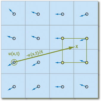
顾名思义，这个方法借鉴了拉格朗日方法的思想。它将网格建模成移动到网格中心点的粒子，根据当前粒子的速度，back trace找到在一个时间步长之前这个粒子所处的位置，并采样该位置的速度作为当前网格的速度。如公式(3.1.3)所示，左边是解析形式，右边是离散形式。

其中 为速度场， 为网格x,y的世界空间坐标， 为back trace移动后找到的最近的左下角网格。 为线性插值权重。

下面这张图直观的展示了这个过程，顶点 back trace了 的距离到达 点，找到绿色方框内的四个最近点并做双线性插值得到速度。

处理完平流，剩下比较难处理的就只有压力了。

压力项需要联立流体不可压缩条件来求解，如公式(3.1.4)所示。

求解它需要用到名为Helmholtz-Hodge 分解的技巧。

任意向量场 可以分解为散度处处为0的场(也就是) 和标量场 的梯度场。

注意看，在公式(3.1.4)我们要求的速度场散度为0，而公式(3.1.5)中的刚好能满足要求！同时，水的压强 也应该是标量，和(3.1.5)中的 对应上。

这意味着令更新前的速度场 为 ，我们可以用公式(3.1.6)的方式求出更新后的速度。

然而，我们仍不知道压力 的值。对此，我们需要在方程(3.1.6)两边求散度，得公式(3.1.7)

由于必须满足 因此，我们得到了只关于 和 的方程(3.1.8)，其中 为在x, y轴上的分量。这里额外提一嘴，这里 这种形式的微分方程便是大名鼎鼎的泊松方程。

公式(3.1.8)本质上是关于 的线性方程组 ，在GPU我们可以用Jacobi迭代求解。（这里提一嘴，在数值分析的角度来看，不是所有线性方程组都能用Jacobi迭代求解，但 是对称正定且主对角占优的，性质相当好，可以放心大胆用Jacobi迭代）

具体来说，设定一个初始值 ，多次迭代计算 直到某个设定的精度终点或迭代次数，单次迭代用如下方式构造：

现在我们已经有了实现流体模拟的所有工具，下面我们可以写出整个算法的伪代码，有兴趣的读者可以照着伪代码实现一遍。

def step():
	advection() #公式(3.1.3)
    solve_viscocity() #公式(3.1.2)
    solve_external_force() #公式(3.1.2)
    for i in range(max_jacobi_iter):
        solve_jacobi() # 公式(3.1.9)
    solve_pressure() # 公式(3.1.6)

下面给出单文件实现（交互代码参考了taichi/python/taichi/examples/simulation/stable_fluid.py at master · taichi-dev/taichi）：

import taichi as ti
import numpy as np

res = 512
ti.init(arch=ti.gpu)

v = ti.Vector.field(2, float, shape=(res, res))
tmp_v = ti.Vector.field(2, float, shape=(res, res))
v_div = ti.field(float, shape=(res, res))
v_curls = ti.field(float, shape=(res, res))
p = ti.field(float, shape=(res, res))
tmp_p = ti.field(float, shape=(res, res))
col = ti.Vector.field(3, float, shape=(res, res))
tmp_col = ti.Vector.field(3, float, shape=(res, res))

dyn = ti.Vector.field(3, float, shape=(res, res))
tmp_dyn = ti.Vector.field(3, float, shape=(res, res))

dt = 0.002
jacobi_iterations = 100
dx = 500.0 / res
mu = 0.02

force_radius = res / 6.0
f_strength = 2000.0 / dt

curl_strength = 0
debug = False

@ti.func
def sample(f :ti.template(), x : ti.i32, y : ti.i32):
    pos = ti.Vector([ti.math.clamp(x, 0, res - 1), ti.math.clamp(y, 0, res - 1)])
    return f[pos[0], pos[1]]

@ti.func
def linear_sample(vf: ti.template(), coord: ti.types.vector(2, ti.f32)):
    ld = ti.cast(ti.math.floor(coord), ti.i32)
    rd = ld + ti.Vector([1, 0])
    lu = ld + ti.Vector([0, 1])
    ru = ld + ti.Vector([1, 1])

    wx = coord[0] - ld[0]
    wy = coord[1] - ld[1]

    return sample(vf, ld[0], ld[1]) * (1 - wx) * (1 - wy) + \
           sample(vf, rd[0], rd[1]) * wx * (1 - wy) + \
           sample(vf, lu[0], lu[1]) * (1 - wx) * wy + \
           sample(vf, ru[0], ru[1]) * wx * wy

@ti.func
def get_pos(i: ti.i32, j: ti.i32):
    return (ti.Vector([i, j]) + 0.5) * dx

@ti.func
def get_coord(pos: ti.types.vector(2, ti.f32)):
    return ti.Vector([ti.math.clamp(pos[0] / dx - 0.5, 0.0, res - 2.0),
                      ti.math.clamp(pos[1] / dx - 0.5, 0.0, res - 2.0)])


@ti.func
def calc_laplaican(i: ti.i32, j: ti.i32, fsrc: ti.template()):
    sum_nb = sample(fsrc, i - 1 , j) + \
             sample(fsrc, i + 1 , j) + \
             sample(fsrc, i, j - 1) + \
             sample(fsrc, i, j + 1)
    return (sum_nb - fsrc[i, j] * 4) / (dx * dx)


@ti.func
def calc_divergence(i: ti.i32, j: ti.i32, fsrc: ti.template()):
    res_x = sample(fsrc, i + 1, j)[0]
    res_x = res_x - sample(fsrc, i - 1, j)[0]
    res_y = sample(fsrc, i, j + 1)[1]
    res_y = res_y - sample(fsrc, i, j - 1)[1]
    return (res_x + res_y) / (2 * dx)


@ti.kernel
def advection(vf: ti.template(), fsrc: ti.template(), fdst: ti.template()):
    for i, j in vf:
        v_ij = sample(vf, i, j)
        p_ij = get_pos(i, j)
        p_ij = p_ij - v_ij * dt
        coord = get_coord(p_ij)
        fdst[i, j] = linear_sample(fsrc, coord)


@ti.kernel
def apply_impulse(vf: ti.template(), dyef: ti.template(), imp_data: ti.types.ndarray()):
    for i, j in vf:
        omx, omy = imp_data[2], imp_data[3]
        mdir = ti.Vector([imp_data[0], imp_data[1]])
        dis_x, dis_y = (i + 0.5 - omx), (j + 0.5 - omy)
        d2 = dis_x * dis_x + dis_y * dis_y
        # dv = F * dt
        factor = ti.exp(-d2 / force_radius)

        dc = sample(dyef, i, j)
        a = dc.norm()

        # momentum = (mdir * f_strength * factor + g_dir * a / (1 + a)) * dt
        momentum = (mdir * f_strength * factor) * dt

        vfield = sample(vf, i, j)
        vf[i, j] = vfield + momentum
        # add dye
        if mdir.norm() > 0.5:
            dc += ti.exp(-d2 * (4 / (res / 15) ** 2)) * ti.Vector([imp_data[4], imp_data[5], imp_data[6]])

        dyef[i, j] = dc




@ti.kernel
def viscosity_and_external_force(fsrc: ti.template(), fdest: ti.template()):
    for i, j in fsrc:
        fdest[i, j] = calc_laplaican(i, j, fsrc) * mu * dt + fsrc[i, j]


@ti.kernel
def solve_pressure_jacobi(psrc: ti.template(), pdst: ti.template(), vf: ti.template()):
    for i, j in psrc:
        p_l = sample(psrc, i - 1, j)#psrc[i - 1 if i > 0 else i, j]
        p_r = sample(psrc, i + 1, j)#psrc[i + 1 if i < res - 1 else i, j]
        p_d = sample(psrc, i, j - 1)#psrc[i, j - 1 if j > 0 else j]
        p_u = sample(psrc, i, j + 1)#psrc[i, j + 1 if j < res - 1 else j]
        div = calc_divergence(i, j, vf)
        pdst[i, j] = (p_l + p_r + p_d + p_u - div * dx * dx) * 0.25


@ti.kernel
def apply_pressure(pf: ti.template(), vf: ti.template()):
    for i, j in pf:
        p_l = sample(pf, i - 1, j)
        p_r = sample(pf, i + 1, j)
        p_d = sample(pf, i, j - 1)
        p_u = sample(pf, i, j + 1)
        vf[i, j] = sample(vf, i, j) - ti.Vector([p_r - p_l, p_u - p_d]) / (2 * dx)


def reset():
    v.fill(0)
    p.fill(0)
    tmp_v.fill(0)
    tmp_p.fill(0)
    dyn.fill(0)


def step(mouse_data):
    global v, tmp_v, p, tmp_p, dyn, tmp_dyn
    advection(v, dyn, tmp_dyn)
    dyn, tmp_dyn = tmp_dyn, dyn
    advection(v, v, tmp_v)
    v, tmp_v = tmp_v, v
    viscosity_and_external_force(v, tmp_v)
    v, tmp_v = tmp_v, v

    apply_impulse(v, dyn, mouse_data)

    for i in range(jacobi_iterations):
         solve_pressure_jacobi(p, tmp_p, v)
         p, tmp_p = tmp_p, p

    apply_pressure(p, v)


class MouseDataGen:
    def __init__(self):
        self.prev_mouse = None
        self.prev_color = None

    def __call__(self, gui):
        # [0:2]: normalized delta direction
        # [2:4]: current mouse xy
        # [4:7]: color
        mouse_data = np.zeros(8, dtype=np.float32)
        if gui.is_pressed(ti.GUI.LMB):
            mxy = np.array(gui.get_cursor_pos(), dtype=np.float32) * res
            if self.prev_mouse is None:
                self.prev_mouse = mxy
                # Set lower bound to 0.3 to prevent too dark colors
                self.prev_color = (np.random.rand(3) * 0.7) + 0.3
            else:
                mdir = mxy - self.prev_mouse
                mdir = mdir / (np.linalg.norm(mdir) + 1e-5)
                mouse_data[0], mouse_data[1] = mdir[0], mdir[1]
                mouse_data[2], mouse_data[3] = mxy[0], mxy[1]
                mouse_data[4:7] = self.prev_color
                self.prev_mouse = mxy
        else:
            self.prev_mouse = None
            self.prev_color = None
        return mouse_data


def main():
    global debug, curl_strength
    visualize_d = True  # visualize dye (default)
    visualize_v = False  # visualize velocity
    visualize_c = False  # visualize curl

    paused = False
    mouse_data = np.zeros(8, dtype=np.float32)

    gui = ti.GUI("Stable Fluid", (res, res))
    md_gen = MouseDataGen()

    while gui.running:
        if gui.get_event(ti.GUI.PRESS):
            e = gui.event
            if e.key == ti.GUI.ESCAPE:
                break
            elif e.key == "r":
                paused = False
                reset()
            elif e.key == "s":
                if curl_strength:
                    curl_strength = 0
                else:
                    curl_strength = 7
            elif e.key == "v":
                visualize_v = True
                visualize_c = False
                visualize_d = False
            elif e.key == "d":
                visualize_d = True
                visualize_v = False
                visualize_c = False
            elif e.key == "c":
                visualize_c = True
                visualize_d = False
                visualize_v = False
            elif e.key == "p":
                paused = not paused
            elif e.key == "b":
                debug = not debug

        if not paused:
            mouse_data = md_gen(gui)
            step(mouse_data)

        if visualize_c:
            # vorticity/curl not computed yet, fall back to dye
            gui.set_image(dyn.to_numpy())
        elif visualize_d:
            gui.set_image(dyn.to_numpy())
        elif visualize_v:
            # single-channel speed map, GUI.set_image does not take 2-channel images
            speed = np.linalg.norm(v.to_numpy(), axis=-1) / dx * dt
            gui.set_image(np.clip(speed * 0.01, 0.0, 1.0))

        gui.show()


if __name__ == "__main__":
    main()

跑出来的效果如下图所示

目前我们默认的jacobi迭代次数设置为100次，看上去很多不是吗。我们可以做个简单小实验，看看不同迭代次数的情况下模拟看上去是什么样的：

	10	20	40	80	160
模拟结果
残差结果()

可以看到相比10次迭代，160次迭代的结果看上去会更清爽一些。10次迭代的结果感觉黏黏的，流体均匀的扩散开了，缺少细节。

从下方的残差对比结果，可以更直观的理解这个问题。迭代次数越少，残差的累积越严重，流体的模拟细节也就越少。

在实际的游戏开发中，我们肯定接受不了上百次迭代，因此我们需要更聪明的算法来计算压力。下面将介绍几个提升解算性能的方法。（到这里其实问题已经聚焦到更快的计算压力项对应的泊松方程/线性方程组，理论上你换别的有助于求解的数值方法【如PCG等】也是ok的，在这篇文献中提供了很多求解泊松方程的算法，感兴趣的读者可以自行查阅）

3.2 DFFT + Stable Fluid

本节将介绍利用离散快速傅里叶变换加速压力项求解的思路。

笔者没有系统学过复分析。因此介绍的知识可能会有很多事实性错误，希望读者包容。

想要将傅里叶变换应用到泊松方程的求解中，需要将公式(3.1.8)做简单变形 ，有公式(3.2.1)和(3.2.2):

公式中 这种对角线上以及贴着最近的两条斜线上为非0元素，其余地方全是0的这种形式的矩阵有个特殊的名字：三对角矩阵，这种矩阵有一些很棒的性质，会在后续的求解过程中用到。 是压力场。

最后带入到公式(3.1.8)中得公式(3.2.3)

是速度的散度场。

对 特征值分解 , 是由单位正交基构成的矩阵， 是对角矩阵( 是实对称的，因此 一定可以在实数域特征值分解)。带入公式(3.2.3)并在两边左乘 并右乘得公式(3.2.4)

公式(3.2.4)的矩阵形式看上去可能很困惑，但事实上对于这个方程很好解。

现在整个 的求解路径开始逐渐清晰起来，我们只剩下一个问题需要解决——如何对 特征值分解。

的特征值分解是有解析解的（推导过程可看附录），结果为：

为第m个特征值， 为第 个特征值对应特征向量的第 维度的数据，也就是矩阵 的m行k列的元素。为了和代码习惯对应上，本文的计数习惯是从0开始的，这里m和k最大到，因此这里的公式可能和你在别的资料中看到的不一致。

观察公式(3.2.7)不难发现 ，因此 是对称的，有

由于是单位正交基组成的，因此有

最后我们能得到，这进一步简化, 的计算为

而FFT擅长快速执行矩阵的乘法计算，我们可以用FFT加速(3.2.8)的计算。

我们先定义离散傅里叶变换。

对于输入信号，我们可以对它做离散傅里叶变换得到对应频域信号

看上去不知所云？我们来做两个操作：

1. 设 同时舍弃 的结果，这意味着我们可以舍弃k, m为0的项。在这个操作之后我们再让k, m从0开始计数。此时原来公式(3.2.9)中的k, m应该对应k+1, m+1
2. 假设我们有 项数据。

将这两个操作应用到(3.2.9)得(3.2.10)

公式(3.2.7)的特征向量神奇的出现在了(3.2.10)的虚部上！这意味着：

对每个维度为N的列向量，我们总可以构造另一个列向量 则

计算矩阵乘法 等价于计算对 做离散傅里叶变换然后取其虚部

这个结论对行向量同样成立。（我们这里实际上是在做0延拓，网上的其它文章可能在这里告诉你要奇延拓，但这里0延拓和奇延拓的结果就差了2倍且计算量没有变化，这两种方法用谁都差不多）

而对离散傅里叶变换，我们有快速离散傅里叶变换 算法加速这个过程！

写到这里，我觉得这部分正文内容有点太多了，所以关于DFFT算法的详细描述放到附录章节了。

有了快速傅里叶变换这块最后的拼图，我们终于可以给出完整的求解过程的伪代码。

def solve_pressure():
	计算速度散度场W(公式3.2.3)
	用快速傅里叶变换计算QWQ(公式3.2.8)
	计算\bar{P}(公式3.2.5)
	用快速傅里叶变换计算P=Q\bar{P}Q(别忘了Q的逆就是Q)

最后给出算法完整的单文件实现。

import taichi as ti
import numpy as np
import math

res = 511   # DST-I 要零填充到 2*(res+1) 再做 2 的幂 FFT，所以 res 必须是 2^k - 1
ti.init(arch=ti.gpu)

v = ti.Vector.field(2, float, shape=(res, res))
tmp_v = ti.Vector.field(2, float, shape=(res, res))
v_div = ti.field(float, shape=(res, res))
v_curls = ti.field(float, shape=(res, res))
# 诊断用：泊松方程的离散残差 r = ∇·v − ∇²p（投影前），以及投影后残留的散度 ∇·v（投影后）
poisson_res = ti.field(float, shape=(res, res))
div_res = ti.field(float, shape=(res, res))
p = ti.field(float, shape=(res, res))
tmp_p = ti.field(float, shape=(res, res))
col = ti.Vector.field(3, float, shape=(res, res))
tmp_col = ti.Vector.field(3, float, shape=(res, res))

dyn = ti.Vector.field(3, float, shape=(res, res))
tmp_dyn = ti.Vector.field(3, float, shape=(res, res))

dt = 0.002
jacobi_iterations = 80
dx = 500.0 / res
mu = 0.02

force_radius = res / 6.0
f_strength = 2000.0 / dt

curl_strength = 0
debug = False

@ti.func
def fft_bit_inverse(i : ti.i32, max_iter : ti.i32):
    # 把 i 的低 max_iter 位反转：每次取最低位拼到结果的低位
    r = 0
    for _ in range(max_iter):
        r = (r << 1) | (i & 1)
        i = i >> 1
    return r

@ti.func
def fft_omega(k : ti.i32, N : ti.i32):
    return ti.Vector([ti.math.cos(2 * ti.math.pi / N * k),
                      ti.math.sin(2 * ti.math.pi / N * k)])


@ti.func
def fft_times_cmplx(w1 : ti.types.vector(2, ti.f32), w2 : ti.types.vector(2, ti.f32)):
    return ti.Vector([w1[0] * w2[0] - w1[1] * w2[1],
                      w1[1] * w2[0] + w1[0] * w2[1]])


@ti.func
def fft_eigen_value(m : ti.i32):
    return 2 * ti.math.cos(ti.cast(m + 1, ti.f32) / (res + 1) * ti.math.pi) - 2

@ti.kernel
def fft_init_2d_y(vdst : ti.template(), vsrc : ti.template(), max_iter : ti.i32):
    for x, y in vsrc:
        vdst[x, y] = vsrc[x, fft_bit_inverse(y, max_iter)]


@ti.kernel
def fft_iteration_2d_y(vsrc : ti.template(), vdst : ti.template(),
                     iter : ti.i32, max_iter : ti.i32, sign : ti.i32):
    for x, y in vsrc:
        N = 1 << iter
        half = 1 << (iter - 1)
        k = y % N

        i0 = y
        m = k
        s = 1
        if k >= half:
            i0 = y - half
            m = k - half
            s = -1
        i1 = i0 + half

        vdst[x, y] = vsrc[x, i0] + s * fft_times_cmplx(vsrc[x, i1], fft_omega(sign * m, N))

@ti.kernel
def fft_init_2d_x(vdst : ti.template(), vsrc : ti.template(), max_iter : ti.i32):
    for x, y in vdst:
        vdst[x, y] = vsrc[fft_bit_inverse(x, max_iter), y]


@ti.kernel
def fft_iteration_2d_x(vsrc : ti.template(), vdst : ti.template(),
                     iter : ti.i32, max_iter : ti.i32, sign : ti.i32):
    for x, y in vsrc:
        N = 1 << iter
        half = 1 << (iter - 1)
        k = x % N

        i0 = x
        m = k
        s = 1
        if k >= half:
            i0 = x - half
            m = k - half
            s = -1
        i1 = i0 + half

        vdst[x, y] = vsrc[i0, y] + s * fft_times_cmplx(vsrc[i1, y], fft_omega(sign * m, N))

tmp_res = res * 2 + 2
tmp_max_iter = int(math.log2(tmp_res))
assert (tmp_res & (tmp_res - 1)) == 0, \
    f"DST-I 要求 2*(res+1) 是 2 的幂，即 res = 2^k - 1；当前 res={res} -> tmp_res={tmp_res}"

fft_tmp_0 = ti.Vector.field(2, float, shape=(tmp_res, tmp_res))
fft_tmp_1 = ti.Vector.field(2, float, shape=(tmp_res, tmp_res))

# 逆 DST 的归一化：S·S = (res+1)/2 · I，两个方向各乘 2/(res+1)
fft_inv_scale = (2.0 / (res + 1)) ** 2


@ti.kernel
def fft_calc_velocity_field(vsrc : ti.template(), vdst : ti.template(),
                            src_res : ti.i32):
    for x,y in vdst:
        if x > 0 and x <= src_res and y > 0 and y <= src_res:
            vdst[x, y] =  ti.Vector([calc_divergence(x - 1, y - 1, vsrc), 0.0])
        else:
            vdst[x, y] = ti.Vector([0.0, 0.0])


@ti.kernel
def fft_solve_in_frequence_field(vsrc : ti.template(), vdst : ti.template()):
    for x,y in vsrc:
        if x > 0 and x <= res and y > 0 and y <= res:
            vdst[x, y] = vsrc[x, y] / (fft_eigen_value(x - 1) + fft_eigen_value(y - 1)) \
                         * (dx * dx) * fft_inv_scale
        else:
            vdst[x, y] = ti.Vector([0.0, 0.0])


@ti.kernel
def fft_apply_end(vsrc : ti.template()):
    for x, y in vsrc:
        if x > 0 and x <= res and y > 0 and y <= res:
            vsrc[x, y] = ti.Vector([vsrc[x, y][1], 0.0])
        else:
            vsrc[x, y] = ti.Vector([0.0, 0.0])


def fft_apply_x(f0, f1):
    fft_init_2d_x(f1, f0, tmp_max_iter)
    f0, f1 = f1, f0                     # 交换后 f0 指向数据所在的那块
    for i in range(1, tmp_max_iter + 1):
        fft_iteration_2d_x(f0, f1, i, tmp_max_iter, 1)
        f0, f1 = f1, f0
    fft_apply_end(f0)
    return f0                           # max_iter 级蝶形结束后落在哪块取决于奇偶，交给调用方

def fft_apply_y(f0, f1):
    fft_init_2d_y(f1, f0, tmp_max_iter)
    f0, f1 = f1, f0
    for i in range(1, tmp_max_iter + 1):
        fft_iteration_2d_y(f0, f1, i, tmp_max_iter, 1)
        f0, f1 = f1, f0
    fft_apply_end(f0)
    return f0


@ti.kernel
def fft_copy_to_p(vsrc : ti.template()):
    # 把 2*(res+1) 网格里 1..res 区块的实部搬回 p
    for i, j in p:
        p[i, j] = vsrc[i + 1, j + 1][0]


def fft_other(f):
    return fft_tmp_1 if f is fft_tmp_0 else fft_tmp_0


def solve_poission(vsrc):
    # 计算散度，填到 2*(res+1) 网格
    fft_calc_velocity_field(vsrc, fft_tmp_0, res)

    # 第一步，正变换
    cur = fft_apply_x(fft_tmp_0, fft_tmp_1)
    cur = fft_apply_y(cur, fft_other(cur))

    # 第二步，在频域解 possion
    nxt = fft_other(cur)
    fft_solve_in_frequence_field(cur, nxt)
    cur = nxt

    # 第三步，从频域变回空域
    cur = fft_apply_x(cur, fft_other(cur))
    cur = fft_apply_y(cur, fft_other(cur))

    fft_copy_to_p(cur)

    


@ti.func
def sample(f :ti.template(), x : ti.i32, y : ti.i32):
    pos = ti.Vector([ti.math.clamp(x, 0, res - 1), ti.math.clamp(y, 0, res - 1)])
    return f[pos[0], pos[1]]

@ti.func
def linear_sample(vf: ti.template(), coord: ti.types.vector(2, ti.f32)):
    ld = ti.cast(ti.math.floor(coord), ti.i32)
    rd = ld + ti.Vector([1, 0])
    lu = ld + ti.Vector([0, 1])
    ru = ld + ti.Vector([1, 1])

    wx = coord[0] - ld[0]
    wy = coord[1] - ld[1]

    return sample(vf, ld[0], ld[1]) * (1 - wx) * (1 - wy) + \
           sample(vf, rd[0], rd[1]) * wx * (1 - wy) + \
           sample(vf, lu[0], lu[1]) * (1 - wx) * wy + \
           sample(vf, ru[0], ru[1]) * wx * wy

@ti.func
def get_pos(i: ti.i32, j: ti.i32):
    return (ti.Vector([i, j]) + 0.5) * dx

@ti.func
def get_coord(pos: ti.types.vector(2, ti.f32)):
    return ti.Vector([ti.math.clamp(pos[0] / dx - 0.5, 0.0, res - 2.0),
                      ti.math.clamp(pos[1] / dx - 0.5, 0.0, res - 2.0)])


@ti.func
def calc_laplaican(i: ti.i32, j: ti.i32, fsrc: ti.template()):
    sum_nb = sample(fsrc, i - 1 , j) + \
             sample(fsrc, i + 1 , j) + \
             sample(fsrc, i, j - 1) + \
             sample(fsrc, i, j + 1)
    return (sum_nb - fsrc[i, j] * 4) / (dx * dx)


@ti.func
def calc_divergence(i: ti.i32, j: ti.i32, fsrc: ti.template()):
    res_x = sample(fsrc, i + 1, j)[0]
    res_x = res_x - sample(fsrc, i - 1, j)[0]
    res_y = sample(fsrc, i, j + 1)[1]
    res_y = res_y - sample(fsrc, i, j - 1)[1]
    return (res_x + res_y) / (2 * dx)


@ti.kernel
def compute_poisson_residual(vf: ti.template(), pf: ti.template(), rf: ti.template()):
    for i, j in rf:
        rf[i, j] = calc_divergence(i, j, vf) - calc_laplaican(i, j, pf)


@ti.kernel
def compute_divergence_field(vf: ti.template(), rf: ti.template()):s
    for i, j in rf:
        rf[i, j] = calc_divergence(i, j, vf)


@ti.kernel
def advection(vf: ti.template(), fsrc: ti.template(), fdst: ti.template()):
    for i, j in vf:
        v_ij = sample(vf, i, j)
        p_ij = get_pos(i, j)
        p_ij = p_ij - v_ij * dt
        coord = get_coord(p_ij)
        fdst[i, j] = linear_sample(fsrc, coord)


@ti.kernel
def apply_impulse(vf: ti.template(), dyef: ti.template(), imp_data: ti.types.ndarray()):
    for i, j in vf:
        omx, omy = imp_data[2], imp_data[3]
        mdir = ti.Vector([imp_data[0], imp_data[1]])
        dis_x, dis_y = (i + 0.5 - omx), (j + 0.5 - omy)
        d2 = dis_x * dis_x + dis_y * dis_y
        # dv = F * dt
        factor = ti.exp(-d2 / force_radius)

        dc = sample(dyef, i, j)
        a = dc.norm()

        # momentum = (mdir * f_strength * factor + g_dir * a / (1 + a)) * dt
        momentum = (mdir * f_strength * factor) * dt

        vfield = sample(vf, i, j)
        vf[i, j] = vfield + momentum
        # add dye
        if mdir.norm() > 0.5:
            dc += ti.exp(-d2 * (4 / (res / 15) ** 2)) * ti.Vector([imp_data[4], imp_data[5], imp_data[6]])

        dyef[i, j] = dc * 0.92




@ti.kernel
def viscosity_and_external_force(fsrc: ti.template(), fdest: ti.template()):
    for i, j in fsrc:
        fdest[i, j] = calc_laplaican(i, j, fsrc) * mu * dt + fsrc[i, j]


@ti.kernel
def solve_pressure_jacobi(psrc: ti.template(), pdst: ti.template(), vf: ti.template()):
    for i, j in psrc:
        p_l = sample(psrc, i - 1, j)#psrc[i - 1 if i > 0 else i, j]
        p_r = sample(psrc, i + 1, j)#psrc[i + 1 if i < res - 1 else i, j]
        p_d = sample(psrc, i, j - 1)#psrc[i, j - 1 if j > 0 else j]
        p_u = sample(psrc, i, j + 1)#psrc[i, j + 1 if j < res - 1 else j]
        div = calc_divergence(i, j, vf)
        pdst[i, j] = (p_l + p_r + p_d + p_u - div * dx * dx) * 0.25


@ti.kernel
def apply_pressure(pf: ti.template(), vf: ti.template()):
    for i, j in pf:
        p_l = sample(pf, i - 1, j)
        p_r = sample(pf, i + 1, j)
        p_d = sample(pf, i, j - 1)
        p_u = sample(pf, i, j + 1)
        vf[i, j] = sample(vf, i, j) - ti.Vector([p_r - p_l, p_u - p_d]) / (2 * dx)


def reset():
    v.fill(0)
    p.fill(0)
    tmp_v.fill(0)
    tmp_p.fill(0)
    dyn.fill(0)


def step(mouse_data):
    global v, tmp_v, p, tmp_p, dyn, tmp_dyn
    advection(v, dyn, tmp_dyn)
    dyn, tmp_dyn = tmp_dyn, dyn
    advection(v, v, tmp_v)
    v, tmp_v = tmp_v, v
    viscosity_and_external_force(v, tmp_v)
    v, tmp_v = tmp_v, v

    apply_impulse(v, dyn, mouse_data)

    solve_poission(v)

    apply_pressure(p, v)


class MouseDataGen:
    def __init__(self):
        self.prev_mouse = None
        self.prev_color = None

    def __call__(self, gui):
        # [0:2]: normalized delta direction
        # [2:4]: current mouse xy
        # [4:7]: color
        mouse_data = np.zeros(8, dtype=np.float32)
        if gui.is_pressed(ti.GUI.LMB):
            mxy = np.array(gui.get_cursor_pos(), dtype=np.float32) * res
            if self.prev_mouse is None:
                self.prev_mouse = mxy
                # Set lower bound to 0.3 to prevent too dark colors
                self.prev_color = (np.random.rand(3) * 0.7) + 0.3
            else:
                mdir = mxy - self.prev_mouse
                mdir = mdir / (np.linalg.norm(mdir) + 1e-5)
                mouse_data[0], mouse_data[1] = mdir[0], mdir[1]
                mouse_data[2], mouse_data[3] = mxy[0], mxy[1]
                mouse_data[4:7] = self.prev_color
                self.prev_mouse = mxy
        else:
            self.prev_mouse = None
            self.prev_color = None
        return mouse_data


def _diverging_image(r):
    # 有符号残差：蓝(负) - 白(零) - 红(正)，用 99 分位做归一化，避免个别边界点把整张图压黑
    hi = float(np.percentile(np.abs(r), 99.0))
    hi = hi if hi > 1e-20 else 1.0
    u = np.clip(r / hi, -1.0, 1.0) * 0.5 + 0.5
    img = np.empty(u.shape + (3,), dtype=np.float32)
    img[..., 0] = np.clip(2.0 * u, 0.0, 1.0)
    img[..., 1] = 1.0 - np.abs(2.0 * u - 1.0)
    img[..., 2] = np.clip(2.0 - 2.0 * u, 0.0, 1.0)
    return img


def _magnitude_image(r):
    # 非负残差：黑 - 红 - 黄 - 白
    hi = float(np.percentile(np.abs(r), 99.0))
    hi = hi if hi > 1e-20 else 1.0
    t = np.clip(np.abs(r) / hi, 0.0, 1.0)
    img = np.empty(t.shape + (3,), dtype=np.float32)
    img[..., 0] = np.clip(1.5 * t, 0.0, 1.0)
    img[..., 1] = np.clip(1.5 * t - 0.5, 0.0, 1.0)
    img[..., 2] = np.clip(1.5 * t - 1.0, 0.0, 1.0)
    return img


def _stats(r):
    a = np.abs(r)
    return f"max {a.max():.2e}  l2 {np.sqrt((r * r).mean()):.2e}"


def main():
    global debug, curl_strength
    view = "d"  # d: dye, v: speed, e: 泊松残差, f: 投影后散度

    paused = False
    mouse_data = np.zeros(8, dtype=np.float32)

    gui = ti.GUI("Stable Fluid", (res, res))
    md_gen = MouseDataGen()

    while gui.running:
        if gui.get_event(ti.GUI.PRESS):
            e = gui.event
            if e.key == ti.GUI.ESCAPE:
                break
            elif e.key == "r":
                paused = False
                reset()
            elif e.key == "s":
                if curl_strength:
                    curl_strength = 0
                else:
                    curl_strength = 7
            elif e.key in ("d", "v", "e", "f"):
                # e: 泊松方程残差 r = ∇·v − ∇²p；f: 投影后残留的 |∇·v|
                view = e.key
            elif e.key == "p":
                paused = not paused
            elif e.key == "b":
                debug = not debug

        if not paused:
            mouse_data = md_gen(gui)
            step(mouse_data)

        if view == "e":
            r = poisson_res.to_numpy()
            gui.set_image(_diverging_image(r))
            gui.text(f"Poisson residual r = div v - lap p    {_stats(r)}",
                     (0.02, 0.02), font_size=14)
        elif view == "f":
            r = div_res.to_numpy()
            gui.set_image(_magnitude_image(r))
            gui.text(f"|div v| after projection    {_stats(r)}",
                     (0.02, 0.02), font_size=14)
        elif view == "v":
            # single-channel speed map, GUI.set_image does not take 2-channel images
            speed = np.linalg.norm(v.to_numpy(), axis=-1) / dx * dt
            gui.set_image(np.clip(speed * 0.01, 0.0, 1.0))
        else:
            gui.set_image(dyn.to_numpy())

        gui.show()


if __name__ == "__main__":
    main()

模拟结果如下

看上去和stable fluid结果差不多，同时耗时似乎也没有承诺的加速？

事实上你估算一下FLOPS, 这种算法的计算量和81次Jacobi迭代相当，而80次Jacobi迭代的结果已经相当可观了。

个人觉得问题出在0-延拓，这个方法将FFT的分辨率翻倍，但没有0-延拓FFT的蝶形结构就会发生变化了，后面肯定要优化，但怎么优化还没想好。

上面那句”0-延拓把分辨率翻倍”和”蝶形结构变了”，值得摊开说一下，因为它同时解释了”为什么没加速”和”能怎么优化”这两件事。

（一）为什么长度会翻倍

公式(3.2.10) 说的是： 维的 矩阵乘法，等价于对 0 延拓后的序列做一次 点的复 DFT 再取虚部。这个 被两个条件同时卡死：

• 要让 基（公式(3.2.7)）恰好落在 DFT 的虚部上，延拓长度必须是 ——分母 来自三对角矩阵特征向量的定义，系数 来自第 项与第 项成对出现；
• 要能用 Cooley-Tukey， 必须是 的幂。

两条合起来即 ，也就是

网格边长只能取 ——取 而不是 的原因就在这里，代码里 tmp_res = res * 2 + 2 和那句 assert (tmp_res & (tmp_res - 1)) == 0 检查的正是这一条。代价是可以量化的：若取 ， 不是 2 的幂，只能硬凑到 ，等于白白多填充 倍。

当 时 ，工作区从 张到 ：每维长度约 2 倍，二维格点数 倍。

但要说清楚，这里的”翻倍”是”变换长度翻倍”，不是”求解精度翻倍”。真正的解只有 那么大，多出来的 个格点全是填充。从频域看， 点频谱里我们只用 这 个频点的虚部，占全部 个频点的

而 与 这两个自对偶模恒为实数，被直接丢掉。换句话说，一半以上的频域信息是”为了凑 DFT 格式而造出来的”，并不承载物理内容。

（二）蝶形结构变成了什么样

标准 Cooley-Tukey 的蝶形图默认输入全非零，因此每层每块都是满的 个非平凡蝶形。0 延拓把一半输入换成了零，破坏的正是这个前提。

把 0 延拓后的 按 bit-reversal 重排，在蝶形网络的输入端（也就是重排之后的那份数组，而非 DFT 的自变量 本身；”bit-reversal + 蝶形网络”整体等于 的自然序 DFT），零元的落点出奇地规整：

即”下标 0 一个，加上全部奇数下标”，共 个（ 时为 513 个）。这一步不需要”连续被打散”的图像化解释，一行就够：bit-reversal 把 的最低位搬到最高位，故

于是 与” 为奇数”等价。 的非零段是下标 （对应 ），剩下的自然是 ，即全部奇数下标，再加 这个落在 的特殊点。

这直接导致第一层（iter=1）的蝶形全部退化。iter=1 时块长 、，旋转因子 ，而每个蝶形的第二支路恰好是 0：

在 下，512 个蝶形一个不落地白算，且后 512 个输出是前 512 个的逐位副本——这一层输出的互异值只有 。这是一条结构性结论：与输入数据无关，只由 0 延拓的位置决定。

那么第 2 层之后呢？这里要说准：浪费并不会”逐层演化”，它是恒定的，而且可以精确算出来。 之前我用”每层不重复值的个数”去数冗余，这个量不是结构量——同一算法只换输入，测出来的比例就完全变了：

输入						说明
等差数列	50%	24%	35%	38%	35%	频域近稀疏，撞出伪重复
随机正态	50%	0%	0%	0%	0%	除首层外无重复
平滑正弦	75%	15%	9%	9%	13%	又一套数值

换用与输入无关的秩来度量就干净了： 点复数组占 个实槽，而输入只有 个实自由度，蝶形又是可逆线性变换、不可能改变秩，所以每一层数组张成的实维数恒等于 ，冗余率逐层恒定：

时 ，十层一模一样（实测 为 、 为 ，与闭式一致）。首层看起来”重复一半”，只是这份恒定冗余最显眼的一种表现形态；到第 2 层以后它分散到复数虚部与共轭对称里，从”逐位相减为零”变成了”秩不够”，但浪费量一个比特都没少。

（三）能怎么优化

按”预期收益 ÷ 实现成本”排，前两项是几行代码的事，中间三项要动 kernel 组织，最后一项才是真正的算法重写。

1. 跳过全零行（确定性，，成本：改循环界）。这个办法压根不在蝶形层面：0 延拓后 恒为零，蝶形 kernel 却老老实实把 1024 行全算完。把遍历范围从 行改成 行，flops 与字节同步减半。而且这件事手上其实已经做了——poisson.py 重构版的工作缓冲是 shape=(n, m) = (511, 1024)，只分配 511 行；而正文这段内联实现是 shape=(tmp_res, tmp_res) = (1024, 1024)。两者一对比，那 就在眼前。

2. 把 的求值式换成 （确定性，f32 精度改善约 ，成本：一行）。这条不是”性能优化”而是”精度优化”，但性价比最高。它与”放大倍数”无关，值得单独说清：，分子分母同乘一个因子并不改变相对误差。真正的问题在 fft_eigen_value 的实现方式——

   # 现状：fft_eigen_value
   def fft_eigen_value(m): return 2 * cos((m + 1) / (res + 1) * pi) - 2

   时 ， 是两个都约等于 2 的数相减得到 ，f32 的 24 位尾数在这里被吃掉约 5 位。实测最低模态 的相对误差 ，解只剩 位有效数字。改成稳定式只需一行：

   def fft_eigen_value(m): return -4.0 * sin(pi * (m + 1) / (2.0 * (res + 1))) ** 2

   同一场景下 相对误差降到 （改善约 ），解回到 位。三组 RHS 实测：最慢模态 位、随机 位、平滑 位。

   补充一句：poisson.py 重构版的 sine_eigenvalue 写成 2.0 - 2.0*cos(...)，是同一类写法的另一种符号，f32 下同样在 处损失约 5 位（实测相对误差 ，改 后 ）。这个修改对重构版同样适用。

1. 打包变换（确定性，，成本：改长度 + 两个 kernel）。把 0 延拓序列 （长 ，）的偶位/奇位分别装进一个复序列的实部/虚部：，长度 。对 跑一次 点 FFT 得到 ，再用

   还原出 点谱的前 个频点，取虚部即得 ，后处理仅 flops/频点。这一路的关键好处是：不需要重推任何蝶形结构——radix-2 DIT 网络原样保留，只是长度从 变成 （层数 ）、行数从 变成 。收益来自两处叠加：蝶形数 （）与足迹 （），合计 。实测输出与原稿 0-延拓口径逐点差 （），与直接矩阵 DST 差 。

   顺带说明：这一项替代了原先我打算分开列的”首层折叠”与”R2C 实变换”两条。原因是”首层折叠”单独做会缺一半输出——跳过 iter=1 后压缩得到的数组恒等于 的偶数下标子序列（实测差 ），只能给出偶数 ；而 DST-I 要 全部，奇数 缺 个，且共轭对称 在 为偶数时把偶数映到偶数、奇数映到奇数，不跨类，补不回来。E/O 打包之所以可行，正因为它把奇偶两类信息同时装进了同一个 FFT。这两件事本来就是同一件事的两个侧面，分开列反而会让人误以为收益可以相乘。

2. 蝶形复用（确定性，，成本：改 kernel 写回方式）。现在 fft_iteration 对 i 全遍历，同一个蝶形的 在前半和后半各算了一遍（两处只差符号）。改成”一个线程算一个蝶形、同时写两个输出”， flops。

3. kernel 融合（上界约 字节流量，成本：工程量大）。当前一次求解要跑 51 个 kernel（fft_calc_velocity_field×1 + bitrev×4 + 蝶形层×40 + fft_apply_end×4 + 频域相除×1 + fft_copy_to_p×1），合计约 1.17 GB／帧 的显存流量，arithmetic intensity 只有 flops/byte——必然是 memory-bound，所以省字节比省 flops 更有效。若按打包后（）每方向 1 个 kernel 做完全融合，字节可压到约 MB，即 的上界。但这是 DRAM 字节的线性外推，没算 方向跨步访问（stride ）的合并损失，实际应打 折，属推测，需在目标 GPU 上 profile。

4. 真·实蝶形 DST-I（推测，在打包之上再 ，成本：重推整个分层结构）。这一项才需要重写蝶形——实旋转因子、实存储、不同的分层不变式，工作量约等于把附录 5.2 再推一遍，而边际收益只有 。所以它排最后，理由不是”收益小”，而是”成本/风险最高，且大头已被打包吃掉“。

按同口径折算，优化项 3 与 6 的合计倍数正是常被引用的那个”约 ”：。但两者可行性天差地别，只有拆开看才有意义。

最后提醒一句：这些倍数不能相乘。 第 1 项与第 3 项在字节上部分重叠——打包之后行长已降为 ，”跳过全零行”的收益就从 掉到约 （只剩 那 ）。

3.3 Fast Eulerian Fluid Simulation In Games Using Poisson Filters

（感谢基于UE4，在移动端高效地应用流体模拟 - 知乎 ）

出自这篇文献。

Fast Eulerian Fluid Simulation In Games Using Poisson Filters

Compact Poisson Filters for Fast Fluid Simulation

和FFT类似，这个方法也是在压力项的求解上做手脚。该方法在Stable Fluid的Jacobi迭代的基础上做了工程化改进。

让我们回顾Stable Fluid求解压力项的离散形式

后续为了计算简单，我们令。

加速求解的手段简单粗暴：手动展开公式(3.3.1)，一次性完成多次迭代的工作。（可以减少rt切换次数，移动端友好）

我们先对 展开一次，观察一下展开后的公式有什么规律：

令 是卷积运算符，公式(3.3.2)可以改写成：

规律开始渐渐显现出来了，设 公式(3.3.3)可以改写成：

由于 的数值是固定的，确定 后我们可以预计算 和而不产生任何运行时实际开销 。

， 对其卷积的计算规模是随 平方上涨的，为了更进一步优化，作者选择对矩阵奇异值分解，并只保留最大的那个奇异值：

这里我们将一个 复杂度的计算分解为两个 复杂度的计算，大大降低了整个计算的复杂度。

这里特别提一句，原文中作者应该没有考虑多次迭代，就一次性通过 计算出来 。考虑到 较小，需要多次迭代的情况笔者这里顺手把丢掉的 项补上了，有需要的小伙伴可以看需求自取。

优化后的压力求解，伪代码类似：

h, sigma, v = precompute_svd() #预计算特征值分解

def solve_pressure():
    apply_kernel_x(v * sqrt(sigma)) # 在x方向做滤波
    apply_kernel_y(h * sqrt(sigma)) # 在y方向做滤波

给出单文件实现：

import taichi as ti
import numpy as np

res = 512
ti.init(arch=ti.gpu)

v = ti.Vector.field(2, float, shape=(res, res))
tmp_v = ti.Vector.field(2, float, shape=(res, res))
v_div = ti.field(float, shape=(res, res))
v_curls = ti.field(float, shape=(res, res))
p = ti.field(float, shape=(res, res))
tmp_p = ti.field(float, shape=(res, res))
col = ti.Vector.field(3, float, shape=(res, res))
tmp_col = ti.Vector.field(3, float, shape=(res, res))

dyn = ti.Vector.field(3, float, shape=(res, res))
tmp_dyn = ti.Vector.field(3, float, shape=(res, res))

dt = 0.002
jacobi_iterations = 160
dx = 500.0 / res
mu = 0.02

force_radius = res / 12.0
f_strength = 4000.0 / dt

curl_strength = 0
debug = False

@ti.func
def sample(f :ti.template(), x : ti.i32, y : ti.i32):
    pos = ti.Vector([ti.math.clamp(x, 0, res - 1), ti.math.clamp(y, 0, res - 1)])
    return f[pos[0], pos[1]]

@ti.func
def linear_sample(vf: ti.template(), coord: ti.types.vector(2, ti.f32)):
    ld = ti.cast(ti.math.floor(coord), ti.i32)
    rd = ld + ti.Vector([1, 0])
    lu = ld + ti.Vector([0, 1])
    ru = ld + ti.Vector([1, 1])

    wx = coord[0] - ld[0]
    wy = coord[1] - ld[1]

    return sample(vf, ld[0], ld[1]) * (1 - wx) * (1 - wy) + \
           sample(vf, rd[0], rd[1]) * wx * (1 - wy) + \
           sample(vf, lu[0], lu[1]) * (1 - wx) * wy + \
           sample(vf, ru[0], ru[1]) * wx * wy

@ti.func
def get_pos(i: ti.i32, j: ti.i32):
    return (ti.Vector([i, j]) + 0.5) * dx

@ti.func
def get_coord(pos: ti.types.vector(2, ti.f32)):
    # clamp to [0, res - 2] so that floor(coord) + 1 stays in bounds
    return ti.Vector([ti.math.clamp(pos[0] / dx - 0.5, 0.0, res - 2.0),
                      ti.math.clamp(pos[1] / dx - 0.5, 0.0, res - 2.0)])


@ti.func
def calc_laplaican(i: ti.i32, j: ti.i32, fsrc: ti.template()):
    sum_nb = sample(fsrc, i - 1 , j) + \
             sample(fsrc, i + 1 , j) + \
             sample(fsrc, i, j - 1) + \
             sample(fsrc, i, j + 1)
    return (sum_nb - fsrc[i, j] * 4) / (dx * dx)


@ti.func
def calc_divergence(i: ti.i32, j: ti.i32, fsrc: ti.template()):
    res_x = sample(fsrc, i + 1, j)[0]
    res_x = res_x - sample(fsrc, i - 1, j)[0]
    res_y = sample(fsrc, i, j + 1)[1]
    res_y = res_y - sample(fsrc, i, j - 1)[1]
    return (res_x + res_y) / (2 * dx)


@ti.kernel
def advection(vf: ti.template(), fsrc: ti.template(), fdst: ti.template()):
    for i, j in vf:
        v_ij = sample(vf, i, j)
        p_ij = get_pos(i, j)
        p_ij = p_ij - v_ij * dt
        coord = get_coord(p_ij)
        fdst[i, j] = linear_sample(fsrc, coord)


@ti.kernel
def apply_impulse(vf: ti.template(), dyef: ti.template(), imp_data: ti.types.ndarray()):
    for i, j in vf:
        omx, omy = imp_data[2], imp_data[3]
        mdir = ti.Vector([imp_data[0], imp_data[1]])
        dis_x, dis_y = (i + 0.5 - omx), (j + 0.5 - omy)
        d2 = dis_x * dis_x + dis_y * dis_y
        # dv = F * dt
        factor = ti.exp(-d2 / force_radius)

        dc = sample(dyef, i, j)
        a = dc.norm()

        # momentum = (mdir * f_strength * factor + g_dir * a / (1 + a)) * dt
        momentum = (mdir * f_strength * factor) * dt

        vfield = sample(vf, i, j)
        vf[i, j] = vfield + momentum
        # add dye
        if mdir.norm() > 0.5:
            dc += ti.exp(-d2 * (4 / (res / 15) ** 2)) * ti.Vector([imp_data[4], imp_data[5], imp_data[6]])

        dyef[i, j] = dc * 0.97


@ti.kernel
def apply_pressure(pf: ti.template(), vf: ti.template()):
    for i, j in pf:
        p_l = sample(pf, i - 1, j)
        p_r = sample(pf, i + 1, j)
        p_d = sample(pf, i, j - 1)
        p_u = sample(pf, i, j + 1)
        vf[i, j] = sample(vf, i, j) - ti.Vector([p_r - p_l, p_u - p_d]) / (2 * dx)

@ti.kernel
def viscosity_and_external_force(fsrc: ti.template(), fdest: ti.template()):
    for i, j in fsrc:
        fdest[i, j] = calc_laplaican(i, j, fsrc) * mu * dt + fsrc[i, j]


support_size = 32  # n：一次滤波等价于 n 次 Jacobi 迭代
kernel_size = support_size * 2 + 1
kernel_cnt = 4

poisson_kernel_x = ti.field(float, shape=(kernel_size, kernel_cnt))
poisson_kernel_y = ti.field(float, shape=(kernel_size, kernel_cnt))
b = ti.field(float, shape=(res, res))
poisson_pressure = ti.field(float, shape=(res, res, kernel_cnt))
poisson_pressure_tmp = ti.field(float, shape=(res, res, kernel_cnt))


def _convolve_L(a):
    """把 (2k+1)^2 的核和 L 做二维卷积，得到 (2k+3)^2 的核。"""
    L = np.zeros((3, 3), dtype=np.float64)
    L[0, 1] = L[1, 0] = L[1, 2] = L[2, 1] = 0.25

    out = np.zeros((a.shape[0] + 2, a.shape[1] + 2), dtype=np.float64)
    for di in (-1, 0, 1):
        for dj in (-1, 0, 1):
            c = L[di + 1, dj + 1]
            if c:
                out[1 + di:1 + di + a.shape[0], 1 + dj:1 + dj + a.shape[1]] += c * a
    return out


def precompute_svd(n=support_size):
    """n 次 Jacobi 迭代的等效滤波器做奇异值分解，只保留最大的奇异值。

    Jacobi 迭代 p <- L ⊗ p + b 的核是 L = 1/4·[[0,1,0],[1,0,1],[0,1,0]]。
    从 p^0 = 0 出发迭代 n 次，得到 p^n = (I + L + ... + L^(n-1)) ⊗ b，
    也就是公式 (3.3.4) 里丢掉 P 项后剩下的那部分，所以一次滤波的系数矩阵
    就是这个几何级数 A（支撑 (2n+1)^2，n 固定可预计算）。
    公式 (3.3.5) 里的 L^n 是 P 的传递项，每帧都从 p = 0 起算时用不到。

    A ≈ σ1·u·v^T，把 σ1 开方各分一份给两边的核：
    x 方向卷 v·√σ1，y 方向卷 u·√σ1，
    于是 O(n^2) 的二维卷积拆成两次 O(n) 的一维卷积。
    """
    size = 2 * n + 1
    A = np.zeros((size, size), dtype=np.float64)
    cur = np.array([[1.0]], dtype=np.float64)  # L^0
    for i in range(n):
        A[n - i:n + i + 1, n - i:n + i + 1] += cur
        cur = _convolve_L(cur)

    u, s, vt = np.linalg.svd(A)
    sqrt_sigma = np.sqrt(s[0:kernel_cnt])


    print(f"svd result : sigma {s}")
    kernel_x = (vt[0:kernel_cnt] * sqrt_sigma[:, None]).T   # (2n+1, rank)
    kernel_y = u[:, 0:kernel_cnt] * sqrt_sigma[None, :]     # (2n+1, rank)
    
    print(f"vt : {vt[0]}, u: {u[:,0]}")
    return kernel_x.astype(np.float32), kernel_y.astype(np.float32)


def init_poisson_kernel(n=support_size):
    kernel_x, kernel_y = precompute_svd(n)
    poisson_kernel_x.from_numpy(kernel_x)
    poisson_kernel_y.from_numpy(kernel_y)


init_poisson_kernel()

@ti.func
def poisson_sample(psrc : ti.template(), x : ti.i32, y : ti.i32, z : ti.i32):
    pos = ti.Vector([ti.math.clamp(x, 0, res - 1), ti.math.clamp(y, 0, res - 1), ti.math.clamp(z, 0, kernel_cnt - 1)])
    return psrc[pos[0], pos[1], pos[2]]


@ti.kernel
def solve_poisson_kernel_x(bsrc : ti.template(), pdst : ti.template()):
    for i, j, kernel_index in bsrc:
        acc = 0.0
        for k in range(-support_size, support_size + 1):
                acc += poisson_sample(bsrc, k + i, j, kernel_index) * poisson_kernel_x[k + support_size, kernel_index]
        pdst[i, j, kernel_index] = acc

@ti.kernel
def solve_poisson_kernel_y(bsrc : ti.template(), pdst : ti.template()):
    for i, j, kernel_index in bsrc:
        acc = 0.0
        for k in range(-support_size, support_size + 1):
            acc += poisson_sample(bsrc, i, k + j, kernel_index) * poisson_kernel_y[k + support_size, kernel_index]
        pdst[i, j, kernel_index] = acc

@ti.kernel
def calc_b(vsrc : ti.template(), bdst : ti.template()):
    for i, j in vsrc:
        # b = -dx^2/4 * ∇·v，即公式 (3.3.1) 里的 b
        bdst[i, j] = -0.25 * dx * dx * calc_divergence(i, j, vsrc)

@ti.kernel
def clear_pressure(pdst: ti.template(), tmpdst : ti.template(), bsrc : ti.template()):
    for i,j,k in pdst:
        pdst[i, j, k] = bsrc[i, j]
        tmpdst[i, j, k] = 0.0

@ti.kernel
def gather_poisson_pressure(pdst : ti.template(), poisson_src : ti.template()):
    for i,j in pdst:
        acc = 0.0
        for k in range(kernel_cnt):
            acc += poisson_src[i, j, k]
        pdst[i, j] = acc

def solve_poisson_filter(vsrc, bdst, pdst):
    """一次滤波完成 n 次 Jacobi 迭代：先算 b，再做 x/y 两次可分离一维卷积。"""
    calc_b(vsrc, bdst)
    clear_pressure(poisson_pressure, poisson_pressure_tmp, bdst)

    solve_poisson_kernel_x(poisson_pressure, poisson_pressure_tmp)
    solve_poisson_kernel_y(poisson_pressure_tmp, poisson_pressure)

    gather_poisson_pressure(pdst, poisson_pressure)


def reset():
    v.fill(0)
    p.fill(0)
    tmp_v.fill(0)
    tmp_p.fill(0)
    dyn.fill(0)


def step(mouse_data):
    global v, tmp_v, p, tmp_p, dyn, tmp_dyn
    advection(v, dyn, tmp_dyn)
    dyn, tmp_dyn = tmp_dyn, dyn
    advection(v, v, tmp_v)
    v, tmp_v = tmp_v, v
    viscosity_and_external_force(v, tmp_v)
    v, tmp_v = tmp_v, v

    apply_impulse(v, dyn, mouse_data)

    solve_poisson_filter(v, b, p)

    apply_pressure(p, v)


class MouseDataGen:
    def __init__(self):
        self.prev_mouse = None
        self.prev_color = None

    def __call__(self, gui):
        # [0:2]: normalized delta direction
        # [2:4]: current mouse xy
        # [4:7]: color
        mouse_data = np.zeros(8, dtype=np.float32)
        if gui.is_pressed(ti.GUI.LMB):
            mxy = np.array(gui.get_cursor_pos(), dtype=np.float32) * res
            if self.prev_mouse is None:
                self.prev_mouse = mxy
                # Set lower bound to 0.3 to prevent too dark colors
                self.prev_color = (np.random.rand(3) * 0.7) + 0.3
            else:
                mdir = mxy - self.prev_mouse
                mdir = mdir / (np.linalg.norm(mdir) + 1e-5)
                mouse_data[0], mouse_data[1] = mdir[0], mdir[1]
                mouse_data[2], mouse_data[3] = mxy[0], mxy[1]
                mouse_data[4:7] = self.prev_color
                self.prev_mouse = mxy
        else:
            self.prev_mouse = None
            self.prev_color = None
        return mouse_data


def main():
    global debug, curl_strength
    visualize_d = True  # visualize dye (default)
    visualize_v = False  # visualize velocity
    visualize_c = False  # visualize curl

    paused = False
    mouse_data = np.zeros(8, dtype=np.float32)

    gui = ti.GUI("Stable Fluid", (res, res))
    md_gen = MouseDataGen()

    while gui.running:
        if gui.get_event(ti.GUI.PRESS):
            e = gui.event
            if e.key == ti.GUI.ESCAPE:
                break
            elif e.key == "r":
                paused = False
                reset()
            elif e.key == "s":
                if curl_strength:
                    curl_strength = 0
                else:
                    curl_strength = 7
            elif e.key == "v":
                visualize_v = True
                visualize_c = False
                visualize_d = False
            elif e.key == "d":
                visualize_d = True
                visualize_v = False
                visualize_c = False
            elif e.key == "c":
                visualize_c = True
                visualize_d = False
                visualize_v = False
            elif e.key == "p":
                paused = not paused
            elif e.key == "b":
                debug = not debug

        if not paused:
            mouse_data = md_gen(gui)
            step(mouse_data)

        if visualize_c:
            # vorticity/curl not computed yet, fall back to dye
            gui.set_image(dyn.to_numpy())
        elif visualize_d:
            gui.set_image(dyn.to_numpy())
        elif visualize_v:
            # single-channel speed map, GUI.set_image does not take 2-channel images
            speed = np.linalg.norm(v.to_numpy(), axis=-1) / dx * dt
            gui.set_image(np.clip(speed * 0.01, 0.0, 1.0))

        gui.show()

if __name__ == "__main__":
    main()

这个方法的结果有点菜，但胜在快的不行。本文没有采用原文只计算最大奇异值，而是保留了前4个奇异值。脑测这样放到游戏引擎里只需要将单通道纹理改成4通道纹理。(图形学最重要的就是看起来对！)

一次pass的开销应该不大，按笔者的公式(3.3.4)应该可以把公式改成多次迭代式的，感兴趣的小伙伴可以试试这样对精度提升有多少。（不过说实话 项 分母上有个 ， 比较大的时候基本就是0了，drop掉应该是合理的 ）。

3.4 Lattice Boltzmann Method

想必读者已经注意到了，N-S方程中，最麻烦的便是压力项的求解，目前本文介绍的大部分工作都在压力项上做文章。而对于欧拉法，想要满足不可压缩约束都不可避免的去求解一个线性方程组。

而LBM方法另辟蹊径，从原理上巧妙绕开了压力项的求解，避免了大型线性系统的求解。LBM方法我个人的理解是构造一个元胞自动机，然后在元胞自动机上定义一系列演化规则，这些规则在宏观上可以推导出NS方程从而满足流体性质。

由于元胞自动机在演化时上一帧的状态只由附近的cell决定，不涉及任何全局的线性系统求解，因此LBM算法特别适合塞给GPU并行计算。

在介绍LBM方法之前，我们首先需要介绍Boltzmann方程。

Boltzmann方程认为，流体在微观上是无数个满足牛顿第二定律的小球运动、相互碰撞，最后在宏观上表现出N-S方程描述的性质，而它则是在微观的牛顿第二定律和宏观的N-S方程之间筑起的一架桥梁。其刻画了这些小球在介观（介观对宏观足够小，对微观足够大）上的统计学性质，这些性质可以推导到宏观上的N-S方程。今年获得菲尔兹奖的邓煜最大的贡献之一，便是证明了微观的牛顿第二定律可以推导出介观的Boltzmann方程，不过作为牛马程序，相比证明，我们更关心具体的算法。

在Boltzmann方程建模的主要对象为粒子的速度分布函数 ，对应在时刻 、位置 处速度为 的粒子的数量。

一般使用Boltzmann transport model描述分布场函数 随时间的演化：

和欧拉视角下的N-S方程(1.2)类似，方程的左边 是平流项， 对应外力，而 类似压力项，对应流体粒子之间的碰撞效应。

想要计算某点处的物理属性，我们只需要对该点处的分布函数对速度积分：

压强也可以用这种方式建模，为：

对于 我们可以建模为类似弱可压缩假设（Bhatnagar-Gross-Krook模型）：设定一个标准密度 ，我们希望流体在没有外力干扰的情况下渐渐恢复到标准密度：

对于标准密度 可以采用Maxwell Boltzmann分布：

其中 为维度数。

LBM方法便是上述Boltzmann 方法的离散版本。LBM方法将流体场每个点建模为朝四周移动的概率密度的分布函数。对于2D情况，每个网格存储了九个方向，上、下、左、右、左上、右上、左下、右下、中心（粒子不动）九个方向的密度（D2Q9）。对于三维情况，则是27个方向(D3Q27)。

在Fast and scalable turbulent flow simulation with two-way coupling 的support material中提供了这种离散方式和原始连续方程是等价的证明（Section 2.2），感兴趣的读者可以自行查阅，这里就不展开了（笔者看不懂）

记每个网格点的第 个方向的速度为 ，密度为 。可以计算离散密度以及动量：

我们同样可以写出(3.4.1)的离散形式(3.4.8)

方程左边有点类似semi-Lagrangian 方法的advection，事实上在代码中我们也可以直接用semi-Lagrangian方法处理这项。

方程的右边外力项 很好理解，在交互的时候给每个点一个外力即可。

计算碰撞项需要的 采用Moment representation in the lattice Boltzmann method on massively parallel hardware 中提到的Maxwell-Boltzmann方程的泰勒展开近似：

其中 是和维度阶数相同的张量，在二维情况下可以认为， 为声速， 认为是网格大小一般设为1， 为对应方向的晶格权重(lattice weight)。对于D2Q9有：

的值推算过程补充到附录 5.1 节中。

上面这些工具足够我们给出LBM方法的朴素实现。

def solve_LBM():
    计算 rho, u # 公式(3.4.7)
    for i in range(Q): #遍历每个方向
        计算平衡质量f_eq # 公式 (3.4.9)
        计算collision # 公式 (3.4.5)
        计算advection

下面给出完整python实现

import numpy as np
import taichi as ti

res = 512
ti.init(arch=ti.gpu)

cs_sqr = 1.0 / 3.0
inv_cs_sqr = 1.0 / cs_sqr         
tau = 0.8                       # 松弛时间，nu = cs2 * (tau - 0.5)
omega = 1.0 / tau

w = ti.field(float, shape=(9,))
w.from_numpy(np.array(
    [4.0 / 9.0, 1.0 / 9.0, 1.0 / 9.0, 1.0 / 9.0, 1.0 / 9.0,
     1.0 / 36.0, 1.0 / 36.0, 1.0 / 36.0, 1.0 / 36.0], dtype=np.float32))

c = ti.Vector.field(2, ti.i32, shape=(9,))
c.from_numpy(np.array(
    [
        [ 0,  0],
        [ 1,  0],
        [ 0,  1],
        [-1,  0],
        [ 0, -1],
        [ 1,  1],
        [-1,  1],
        [ 1, -1],
        [-1, -1],
    ], dtype=np.int32))

# 反向方向索引，用于边界反弹
opp = ti.field(ti.i32, shape=(9,))
opp.from_numpy(np.array([0, 3, 4, 1, 2, 7, 8, 5, 6], dtype=np.int32))

f = ti.field(float, shape=(res, res, 9))
tmp_f = ti.field(float, shape=(res, res, 9))

rho = ti.field(float, shape=(res, res))
u = ti.Vector.field(2, float, shape=(res, res))
curl = ti.field(float, shape=(res, res))

dyn = ti.Vector.field(3, float, shape=(res, res))
tmp_dyn = ti.Vector.field(3, float, shape=(res, res))

lbm_substeps = 24       # 每个渲染帧推进几个 lattice 步，决定烟看起来多快
impulse_radius = 24.0   # 交互半径（格子）
dye_radius = 30.0       # 染料注入半径（格子）
dye_strength = 0.5      # 单帧染料注入强度
impulse_speed = 0.1   # 单帧速度增量（lattice 单位，稳定区间约 0.01 ~ 0.1）
u_limit = 0.15          # 局部速度上限，防止持续拖拽把湍流能量堆到发散
dye_decay = 0.999


@ti.func
def sample(vf: ti.template(), x: ti.i32, y: ti.i32):
    pos = ti.Vector([ti.math.clamp(x, 0, res - 1), ti.math.clamp(y, 0, res - 1)])
    return vf[pos[0], pos[1]]


@ti.func
def linear_sample(vf: ti.template(), coord: ti.types.vector(2, ti.f32)):
    ld = ti.cast(ti.math.floor(coord), ti.i32)
    rd = ld + ti.Vector([1, 0])
    lu = ld + ti.Vector([0, 1])
    ru = ld + ti.Vector([1, 1])

    wx = coord[0] - ld[0]
    wy = coord[1] - ld[1]

    return sample(vf, ld[0], ld[1]) * (1 - wx) * (1 - wy) + \
           sample(vf, rd[0], rd[1]) * wx * (1 - wy) + \
           sample(vf, lu[0], lu[1]) * (1 - wx) * wy + \
           sample(vf, ru[0], ru[1]) * wx * wy


@ti.func
def f_eq(k: ti.i32, r: ti.f32, uu: ti.types.vector(2, ti.f32)):
    ci = ti.cast(c[k], ti.f32)

    # u^TQu 
    # = u^T(cici^T - cs^2 I)u 
    # = u^Tcici^Tu - cs^2  u^TIu
    # = dot(u, ci)^2 - cs^2 dot(u, u) 
    cu = ci[0] * uu[0] + ci[1] * uu[1]
    return w[k] * r * (1.0
                       + inv_cs_sqr * cu
                       + 0.5 * inv_cs_sqr * inv_cs_sqr * cu * cu
                       - 0.5 * inv_cs_sqr * (uu[0] * uu[0] + uu[1] * uu[1]))


@ti.kernel
def apply_impulse(f: ti.template(), rho_f: ti.template(), uf: ti.template(),
                  dyef: ti.template(), imp_data: ti.types.ndarray()):
    cx, cy = imp_data[2], imp_data[3]
    du0 = ti.Vector([imp_data[0], imp_data[1]]) * impulse_speed

    r = ti.max(impulse_radius, dye_radius)
    i0 = ti.max(ti.cast(cx - r, ti.i32) - 1, 0)
    i1 = ti.min(ti.cast(cx + r, ti.i32) + 2, res)
    j0 = ti.max(ti.cast(cy - r, ti.i32) - 1, 0)
    j1 = ti.min(ti.cast(cy + r, ti.i32) + 2, res)

    for i, j in ti.ndrange((i0, i1), (j0, j1)):
        ox = i + 0.5 - cx
        oy = j + 0.5 - cy
        d2 = ox * ox + oy * oy
        # 高斯核，边缘衰减到 ~1%
        kern = ti.exp(-4.5 * d2 / (impulse_radius * impulse_radius))
        du = du0 * kern
        r_ij = rho_f[i, j]
        u_old = uf[i, j]

        # 限速：偏离平衡态太远 BGK 会发散
        speed_after = (u_old + du).norm()
        if speed_after > u_limit:
            du = du * (u_limit / speed_after)

        # 把该点的平衡态速度从 u_old 平移到 u_old + du：
        #   f_i <- f_i + f_eq(rho, u+du) - f_eq(rho, u)
        # 质量不变，动量精确增加 rho*du，高阶矩也跟着重新平衡（不会炸出强声波）
        u_new = u_old + du
        for k in ti.static(range(9)):
            f[i, j, k] += f_eq(k, r_ij, u_new) - f_eq(k, r_ij, u_old)

        # 染料
        dye_kern = ti.exp(-4.5 * d2 / (dye_radius * dye_radius))
        dc = dyef[i, j] + dye_strength * dye_kern * ti.Vector([imp_data[4], imp_data[5], imp_data[6]])
        dyef[i, j] = ti.min(dc, 1.0)


@ti.kernel
def advect(fdst: ti.template(), fsrc: ti.template()):
    for x, y, k in fsrc:
        sx = x - c[k][0]
        sy = y - c[k][1]
        if 0 <= sx < res and 0 <= sy < res:
            fdst[x, y, k] = fsrc[sx, sy, k]
        else:
            fdst[x, y, k] = fsrc[x, y, opp[k]]


@ti.kernel
def calc_rho_and_u(rho_dst: ti.template(), vdst: ti.template(), fsrc: ti.template()):
    for x, y in rho_dst:
        r = 0.0
        mem = ti.Vector([0.0, 0.0])
        for k in ti.static(range(9)):
            fk = fsrc[x, y, k]
            r += fk
            mem += fk * ti.cast(c[k], ti.f32)

        rho_dst[x, y] = r
        vdst[x, y] = mem / ti.max(r, 1e-8)


@ti.kernel
def collide(fdst : ti.template(), fsrc: ti.template(), rho_src: ti.template(), usrc: ti.template()):
    for x, y, k in fdst:
        r = rho_src[x, y]
        uu = usrc[x, y]
        fi = fsrc[x, y, k]
        fdst[x, y, k] = fi + omega * (f_eq(k, r, uu) - fi)


@ti.kernel
def advect_dye(usrc: ti.template(), fsrc: ti.template(), fdst: ti.template()):
    for i, j in fdst:
        # lattice 单位：位置用格子坐标，位移 = u * 本帧推进的步数
        p = ti.Vector([i + 0.5, j + 0.5]) - usrc[i, j] * lbm_substeps
        coord = ti.Vector([ti.math.clamp(p[0] - 0.5, 0.0, res - 2.0),
                           ti.math.clamp(p[1] - 0.5, 0.0, res - 2.0)])
        fdst[i, j] = linear_sample(fsrc, coord) * dye_decay


@ti.kernel
def calc_curl(usrc: ti.template(), cf: ti.template()):
    for i, j in cf:
        dy = (sample(usrc, i + 1, j)[1] - sample(usrc, i - 1, j)[1]) * 0.5
        dx = (sample(usrc, i, j + 1)[0] - sample(usrc, i, j - 1)[0]) * 0.5
        cf[i, j] = dy - dx


@ti.kernel
def init_f():
    for x, y, k in f:
        f[x, y, k] = w[k]
        tmp_f[x, y, k] = w[k]
        rho[x, y] = 1.0


def reset():
    u.fill(0)
    dyn.fill(0)
    tmp_dyn.fill(0)
    curl.fill(0)
    init_f()


def step(mouse_data):
    global f, tmp_f, dyn, tmp_dyn

    apply_impulse(f, rho, u, dyn, mouse_data)

    for _ in range(lbm_substeps):
        # 平流
        advect(tmp_f, f)
        f, tmp_f = tmp_f, f
        # 计算密度和速度
        calc_rho_and_u(rho, u, f)
        # 处理碰撞
        collide(tmp_f, f, rho, u)
        f, tmp_f = tmp_f, f

    advect_dye(u, dyn, tmp_dyn)
    dyn, tmp_dyn = tmp_dyn, dyn
    calc_curl(u, curl)


class MouseDataGen:
    def __init__(self):
        self.prev_mouse = None
        self.prev_color = None

    def __call__(self, gui):
        # [0:2]: normalized delta direction
        # [2:4]: current mouse xy
        # [4:7]: color
        mouse_data = np.zeros(8, dtype=np.float32)
        if gui.is_pressed(ti.GUI.LMB):
            mxy = np.array(gui.get_cursor_pos(), dtype=np.float32) * res
            if self.prev_mouse is None:
                self.prev_mouse = mxy
                # Set lower bound to 0.3 to prevent too dark colors
                self.prev_color = (np.random.rand(3) * 0.7) + 0.3
            else:
                mdir = mxy - self.prev_mouse
                mdir = mdir / (np.linalg.norm(mdir) + 1e-5)
                mouse_data[0], mouse_data[1] = mdir[0], mdir[1]
                mouse_data[2], mouse_data[3] = mxy[0], mxy[1]
                mouse_data[4:7] = self.prev_color
                self.prev_mouse = mxy
        else:
            self.prev_mouse = None
            self.prev_color = None
        return mouse_data


def main():
    visualize_d = True   # 染料
    visualize_v = False  # 速度
    visualize_c = False  # 涡量
    visualize_f = False

    paused = False
    mouse_data = np.zeros(8, dtype=np.float32)

    reset()   # f 初始化为 w[k]（rho=1 的平衡态），否则首帧 rho=0，扰动加不进去

    gui = ti.GUI("LBM Fluid", (res, res))
    md_gen = MouseDataGen()

    while gui.running:
        if gui.get_event(ti.GUI.PRESS):
            e = gui.event
            if e.key == ti.GUI.ESCAPE:
                break
            elif e.key == "r":
                paused = False
                reset()
            elif e.key == "v":
                visualize_v = True
                visualize_c = False
                visualize_d = False
                visualize_f = False
            elif e.key == "d":
                visualize_d = True
                visualize_v = False
                visualize_c = False
                visualize_f = False
            elif e.key == "c":
                visualize_c = True
                visualize_d = False
                visualize_v = False
                visualize_f = False
            elif e.key == "p":
                paused = not paused
            elif e.key == "f":
                visualize_f = True
                visualize_c = False
                visualize_d = False
                visualize_v = False

        if not paused:
            mouse_data = md_gen(gui)
            step(mouse_data)

        if visualize_c:
            cf = np.clip(curl.to_numpy() * 8.0, -1.0, 1.0)
            img = np.stack([np.clip(cf, 0, 1), np.zeros_like(cf), np.clip(-cf, 0, 1)], axis=-1)
            gui.set_image(img)
        elif visualize_v:
            speed = np.clip(np.linalg.norm(u.to_numpy(), axis=-1) * 4.0, 0.0, 1.0)
            gui.set_image(np.stack([speed, speed, speed], axis=-1))
        elif visualize_f:
            fnp = np.clip(f.to_numpy().sum(axis=-1) * 0.5, 0.0, 1.0)
            gui.set_image(np.stack([fnp, fnp, fnp], axis=-1))
        else:
            gui.set_image(np.clip(dyn.to_numpy(), 0.0, 1.0))

        gui.show()


if __name__ == "__main__":
    main()

模拟结果如下图所示

LBM方法流体的涡旋细节保留的还是很不错的，然而，可能是因为模拟尺度的原因，它模拟的流体场移动比较慢。

朴素LBM方法最大的问题便是它需要的存储空间实在太多，相比之前介绍的Stable Fluid方法，D2Q9 需要个元素存储分布函数 ，而D3Q27则需要惊人的 ! 算上模拟时使用的ping-pong buffer，需要的存储空间来到了 和。

后续的 Moment representation in the lattice Boltzmann method on massively parallel hardware ，以及High-Order Moment-Encoded Kinetic Simulation of Turbulent Flows 则是在moment 空间的基础上尝试优化LBM方法需要的内存大小。这些方法使用0阶，1阶，2阶矩（一个函数的 阶矩就是， 0阶矩即）来表示完整的分布函数 ，在运行时尝试重建 并计算(有点类似全局光照SH压缩低频环境光的思路)。

3.5 浅水方程

出自Real-time simulation of large bodies of water with small scale details（ACM SIGGRAPH / Eurographics Symposium on Computer Animation, 2010）。本节浅水方程的推导脉络，以及「网格管大尺度水面、粒子管亚网格细节」的耦合思路，均出自该文。

前面几节都在解完整 N-S 方程，对流体内部分得很细；但游戏里的大片水域（湖泊、海洋）只关心水面波纹——丢块石头激起浪花，水底怎样并不重要。

下面按「从 N-S 推到 SWE → SWE 怎么离散 → 伪代码 → 完整实现」的顺序走。

（1）从 N-S 方程到浅水方程

三维不可压 N-S 方程是

它的未知量是三维速度场，每步都得遍历整个水体。

浅水方程用三条假设把它压成二维。先记水面高程 、水深 、底面高程 ：

与时间无关（代码里 H = 12 是一块方框障碍），sample_h_rest = max(h_rest - H, 0) 截到 0 的地方就是露出水面的干地。

第一条是静水压假设：垂直加速度远小于重力，垂直动量方程只剩一项平衡，压强被解成”上方压着多高的水”，

取 向上、水面处相对压强为 0， 就只依赖 与 ，与水平流动解耦。

第二条是水平尺度远大于水深： 时垂直加速度相对重力只有 ，丢掉它正是 (3.5.3) 成立的理由（论文所述；1% 属推测）。

第三条是速度沿水深均匀： 只依赖 ，水柱整体平移，于是可以沿 积分。

对 沿 从 积到 ：上下界随界面移动贡献的两项，正好被自由面运动学条件与不可穿透底面消掉，只剩

通量是 而非 ——水柱越厚，同流速搬的水越多，这是 SWE 与常密度 N-S 的关键差别。

水平动量方程代入 (3.5.3)，压强梯度积掉 后只剩水面坡度，

(3.5.4) 与 (3.5.5) 就是浅水方程；深度平均本会多出底摩擦、非线性修正等项，论文与实现都一并丢掉。

这两条式子点出了 SWE 相对 Stable Fluid 最大的便宜：压力梯度等价于水面坡度 ，压力成了 的显式函数，不必再解泊松方程——它能一帧跑几百子步就靠这个（论文所述）。

再把两式在静止水面附近线性化（设 、丢掉二阶小量），消去速度得

相速与波数无关，即非色散：长短波同速、波形不会被拉散（深水波的 就不是这样）。代入 、 得 m/s，后面定时间步要用。

（2）离散化：交错网格上的显式格式

h 是 、u 是 、v 是 ： 存格心， 存竖边， 存横边， 个格子正好 条边，这叫 Arakawa C 网格（论文所述）。

全放格心会出事： 只能跨两格差分，而逐格交替的模态 在 、 上取值相同、相减为 0——它能任意长在 上却不产生流动，这就是棋盘格振荡。交错后差分只跨一格，该模态重新进入动力学、能被正常衰减（论文所述；代入核对属本文实现）。

连续方程：dhdt_ij 是 (3.5.4) 的中心差分，但 在边上、 在格心，通量里的 要按速度符号取上风侧，

即 sample_h_line；不用两侧平均，因为中心插值在干湿交界处会非物理过冲（本文实现）。

动量方程：代码把对流项也丢了（小振幅低速振荡下是二阶小量，陡化对波纹无益还要付稳定代价），于是

即 dudt_ij10：右端正好是这条边左右两格心的 之差， 在边上、不用插值。

边界吸收层：计算域有界，波撞到最外圈会全反射回来叠成驻波，所以在最外 圈铺抛物线阻尼

边界格上代码连做两次阻尼：


不是笔误，两个分支串行各松弛一次；速度系数是 而非 ，壁面处阻尼率为 0、外缘最强，与海绵层”贴壁最强”的方向相反，所以反射压不干净（本文实现）。

是边界记忆项，把外向流量的散度累积起来、衰减得很快：

、lamdba_decay（原稿拼写，照抄不改），所以它只对”正在往外冲”的波起作用；decay 必须落在 ，否则 指数累积直入水位（本文实现）。层内积分 m，往返反射率 ，吸收只有 23%，只能算”显著抑制”（推测，一维估算）。

粒子耦合：网格管大尺度水面，粒子管亚网格细节（论文所述）。每颗粒子体积 ，落到水面以下即死亡，把体积与体积加权动量记进所在格的 dparticle，再由 particle_apply() 兑现：

前者体积守恒，后者动量守恒（两个质量的加权平均）。它写的是 h 而非 h1，而每子步开头 copy() 都执行 h ← h1，所以粒子抬升不跨子步累积（本文实现）。

时间步：显式格式要求一步内波不跨过一格， s、 m 对应 Courant ，余量很大；max_vel = dx/dt*0.5 不是 CFL 系数，而是速度钳制上限。

（3）伪代码

每帧:
    for _ in range(step):                 # step = int(1e-2/dt) = 10 个子步
        substep()

def substep():
    copy()                                # 双缓冲 *1 → *，清零 dparticle
    solve()                               # 连续 + 动量 + 边界阻尼 + 钳制
    particle_sim()                        # 粒子下落；落水者把体积/动量写入 dparticle
    particle_apply()                      # 抬水位、按质量加权改速度
    diffusion(diffusion_alpha)            # 四邻平均降噪，只影响本帧末子步

def solve():
    for i, j in 所有格心:
        h_ij = h[i,j] - dt/dx * [ h_up(i+½,j)u(i+½,j) - h_up(i-½,j)u(i-½,j)
                                + h_up(i,j+½)v(i,j+½) - h_up(i,j-½)v(i,j-½) ]  # (3.5.7)
        u_ij = u[i+1,j] - g*dt/dx * (eta[i+1,j] - eta[i,j])                    # (3.5.8)
        v_ij = v[i,j+1] - g*dt/dx * (eta[i,j+1] - eta[i,j])
        if 在边界层: σ 阻尼、φ 记忆项，φ ← 0.9 * φ                            # (3.5.9)-(3.5.12)
        h1[i,j]   = max(h_ij, 0)                                              # 水位不许为负
        u1[i+1,j] = clamp(u_ij, ±max_vel)                                     # 速度钳制

下面是完整实现。

import taichi as ti
import numpy as np

ti.init(arch=ti.gpu) # Try to run on GPU

n_field = 512
n_border = 10

pixels = ti.Vector.field(3, dtype=ti.u8, shape=(n_field, n_field))

h = ti.field(dtype=float, shape=[n_field, n_field])
# 在每个网格边上存储速度信息
u = ti.field(dtype=float, shape=[n_field + 1, n_field])
v = ti.field(dtype=float, shape=[n_field, n_field + 1])
# TODO phi 只在边界区域内有效，没必要设置这么大
phi = ti.field(dtype=float, shape=[n_field, n_field])

h1 = ti.field(dtype=float, shape=[n_field, n_field])
# 在每个网格边上存储速度信息
u1 = ti.field(dtype=float, shape=[n_field + 1, n_field])
v1 = ti.field(dtype=float, shape=[n_field, n_field + 1])
# TODO phi 只在边界区域内有效，没必要设置这么大
phi1 = ti.field(dtype=float, shape=[n_field, n_field])

# 扩散（降噪）用的临时缓冲，避免原地读写导致的数据竞争
h_diff = ti.field(dtype=float, shape=[n_field, n_field])
u_diff = ti.field(dtype=float, shape=[n_field + 1, n_field])
v_diff = ti.field(dtype=float, shape=[n_field, n_field + 1])


dt = 1e-3
step = int(1e-2/ dt)
lambda_update = 0.5
lamdba_decay = 0.9
dx = 1e-1

# 扩散系数：0 表示不扩散，越接近 1 平滑越强
diffusion_alpha = 0.2

max_vel = dx / dt * 0.5

g = 10
h_rest = 3
H = 12

HalfCoord = ti.types.struct(
    x=ti.i32,        
    y=ti.i32,        
    fx=ti.i32, # 0或1，表示x是否加了1/2        
    fy=ti.i32  # 0或1，表示y是否加了1/2     
)

c_deposit = 4.0 / 3.0 * ti.math.pi

Particle = ti.types.struct(
    r= ti.float32,
    x= ti.types.vector(3, ti.float32),
    v = ti.types.vector(3, ti.float32)
)

n_max_particle_count = 10000
particles = Particle.field(shape=n_max_particle_count)
particles1 = Particle.field(shape=n_max_particle_count)
# 记录当前粒子数量的常熟
particle_count = ti.field(dtype=ti.int32, shape=2)
# 每帧由于粒子引起的变化量, x 体积变化, y,z 动量变化
dparticle = ti.Vector.field(3, dtype=ti.float32, shape=(n_field, n_field))


@ti.func
def particle_volume(p : Particle):
    return p.r * p.r * p.r * c_deposit


@ti.func
def get_half_coord(x : int, y : int, fx : int, fy : int):
    x += ti.math.floor(fx * 0.5)
    y += ti.math.floor(fy * 0.5)
    fx = fx - ti.math.floor(fx * 0.5) * 2
    fy = fy - ti.math.floor(fy * 0.5) * 2
    return HalfCoord(x=x, y=y, fx=fx, fy=fy)

@ti.func
def print_half_coord(coord: HalfCoord):
    print(f"(x={coord.x}, y={coord.y}, fx={coord.fx}, fy={coord.fy})")

@ti.kernel
def test_half_coord():
    print_half_coord(get_half_coord(1, 2, 0, 0)) # 1, 2, 0, 0
    print_half_coord(get_half_coord(1, 2, 1, 0)) # 1, 2, 1, 0
    print_half_coord(get_half_coord(1, 2,-1, 0)) # 0, 2, 1, 0
    print_half_coord(get_half_coord(1, 2, 0, 1)) # 1, 2, 0, 1
    print_half_coord(get_half_coord(1, 2, 0,-1)) # 1, 1, 0, 1
    print_half_coord(get_half_coord(0, 0,-1, 0)) 


test_half_coord()

@ti.kernel
def initialize():
    for i,j in h:
        h1[i, j] = sample_h_rest(i, j)
        u1[i + 1, j] = 0
        v1[i, j + 1] = 0
        phi1[i, j] = 0
    particle_count[0] = 0
    

@ti.kernel
def copy():
    for i,j in h:
       h[i, j] = h1[i, j]
       v[i, j] = v1[i, j]
       u[i, j] = u1[i, j]
       phi[i, j] = phi1[i, j]
       dparticle[i, j] = ti.Vector([0, 0, 0])

    for pi in particles:
        if pi < particle_count[1]:
            particles[pi] = particles1[pi]
            particle_count[0] = particle_count[1]

@ti.func
def sample_h_rest(x : int, y : int):
    return ti.math.max(h_rest - sample_H(x, y), 0)

@ti.func
def sample_H(x : int, y : int):
    rv = 0.0
    if x > 200 and x < 300 and y > 200 and y < 300:
        rv = H
    return rv

@ti.func
def sample_h(x : int, y : int):
    return h[ti.math.clamp(x, 0, n_field - 1), ti.math.clamp(y, 0, n_field - 1)]

@ti.func
def is_wall(x : int, y : int, fx : int, fy : int):
    coord = get_half_coord(x, y, fx, fy)
    x = coord.x
    y = coord.y
    fx = coord.fx
    fy = coord.fy
    rv = 0

    if coord.fx != 0:
        if (sample_h(x, y) < 1e-4 * dx and sample_H(x, y) > sample_eta(x + 1, y))\
            or (sample_h(x + 1, y) < 1e-4 * dx and sample_H(x + 1, y) > sample_eta(x, y)):
            rv = 1
    if coord.fy != 0:
        if (sample_h(x, y) < 1e-4 * dx and sample_H(x, y) > sample_eta(x, y + 1))\
            or (sample_h(x, y + 1) < 1e-4 * dx and sample_H(x, y + 1) > sample_eta(x, y)):
            rv = 1

    return rv
    

@ti.func
def sample_eta(x : int, y : int):
    return sample_h(x, y) + sample_H(x, y)

@ti.func
def is_border_h(x : int, y : int):
    rv = 0
    if x < n_border or x >= n_field - n_border + 1:
        rv = 1
    return rv

@ti.func
def is_border_v(x : int, y : int):
    rv = 0
    if y < n_border or y >= n_field - n_border + 1:
        rv = 1
    return rv

@ti.func
def sample_sigma_h(x : int, y : int):
    r = ti.math.min(x, n_field - x - 1, n_border)
    return (1.0 - r * r / (n_border * n_border))

@ti.func
def sample_sigma_v(x : int, y : int):
    r = ti.math.min(y, n_field - y - 1, n_border)
    return (1.0 - r * r / (n_border * n_border))

@ti.func
def sample_phi(x : int, y : int):
    return phi[ti.math.clamp(x, 0, n_field - 1), ti.math.clamp(y, 0, n_field - 1)]


@ti.func
def particle_coord(p : Particle):
    return ti.Vector([int(p.x[0]), int(p.x[1])])

@ti.func
def sample_u(x : int, y : int, fx : int, fy : int):
    coord = get_half_coord(x, y, fx, fy)
    return u[coord.x + coord.fx, coord.y]

@ti.func
def sample_v(x : int, y : int, fx : int, fy : int):
    coord = get_half_coord(x, y, fx, fy)
    return v[coord.x, coord.y + coord.fy]

@ti.func
def sample_h_line(x : int, y : int, fx : int, fy : int):
    res = 0.0
    coord = get_half_coord(x, y, fx, fy)
    if coord.fx != 0:
        u_xy = sample_u(x, y, fx, fy)
        if u_xy > 0:
            res = sample_h(coord.x, coord.y)
        else:
            res = sample_h(coord.x + 1, coord.y)
    
    if coord.fy != 0:
        v_xy = sample_v(x, y, fx, fy)
        if v_xy > 0:
            res = sample_h(coord.x, coord.y)
        else:
            res = sample_h(coord.x, coord.y + 1)
    return res

@ti.kernel
def solve():
    for i,j in h:
        # 更新h
        
        dhdt_ij = -(sample_h_line(i, j, 1, 0) * sample_u(i, j, 1, 0) - sample_h_line(i, j, -1, 0) * sample_u(i, j, -1, 0) 
                 + sample_h_line(i, j, 0, 1) * sample_v(i, j, 0, 1) - sample_h_line(i, j, 0, -1) * sample_v(i, j, 0, -1))  / dx
        h_ij = h[i, j] + dhdt_ij * dt

        # 更新u和v
        dudt_ij10 = - g / dx * (sample_eta(i + 1, j) - sample_eta(i, j))
        dudt_ij01 = - g / dx * (sample_eta(i, j + 1) - sample_eta(i, j))

        u_ij = u[i + 1, j] + dudt_ij10 * dt
        v_ij = v[i, j + 1] + dudt_ij01 * dt

        if is_border_h(i, j) != 0:
            sigma_ij = sample_sigma_h(i, j)
            phi_ij = sample_phi(i, j)

            phi_i1j = sample_phi(i + 1, j)
            h_ij += (- sigma_ij * (h_ij - sample_h_rest(i, j)) + phi_ij) * dt
            u_ij += - 0.5 * (phi_i1j + phi_ij) * u_ij * dt
            phi_ij += - lambda_update * sigma_ij * (sample_v(i, j, 0, 1) - sample_v(i, j, 0, -1)) / dx * dt
            phi_ij *= lamdba_decay

            phi1[i, j] = phi_ij
        elif is_border_v(i, j) != 0:
            sigma_ij = sample_sigma_v(i, j)
            phi_ij = sample_phi(i, j)

            phi_ij1 = sample_phi(i, j + 1)
            h_ij += (- sigma_ij * (h_ij - sample_h_rest(i, j)) + phi_ij) * dt
            v_ij += - 0.5 * (phi_ij1 + phi_ij) * v_ij * dt
            phi_ij += - lambda_update * sigma_ij * (sample_u(i, j, 1, 0) - sample_v(i, j, -1, 0)) / dx * dt
            phi_ij *= lamdba_decay

            phi1[i, j] = phi_ij

        if is_border_h(i, j) != 0 or is_border_v(i, j) != 0:
            sigma_ij = ti.math.max(sample_sigma_h(i, j), sample_sigma_v(i, j))

            h_ij += (sample_h_rest(i, j) - h_ij) * sigma_ij * dt
            u_ij -= (1.0 - sigma_ij) * u_ij * dt
            v_ij -= (1.0 - sigma_ij) * v_ij * dt

        h1[i, j] = ti.math.max(h_ij, 0.0)
        
        if is_wall(i, j, 1, 0) == 0:
            u1[i + 1, j] = ti.math.clamp(u_ij, -max_vel, max_vel) 
        
        if is_wall(i, j, 0, 1) == 0:
            v1[i, j + 1] = ti.math.clamp(v_ij, -max_vel, max_vel)

@ti.kernel
def particle_sim():
    for pi in particles:
        if pi < particle_count[0]:
            p = particles[pi]

            p.x += dt * p.v
            p.v += dt * ti.Vector([0, 0, -g])

            p_coord = particle_coord(p)
            if p_coord[0] >= 0 and p_coord[0] < n_field and p_coord[1] >= 0 and p_coord[1] < n_field:
                h_p = h[p_coord]
                if h_p >= p.x[2]:
                    # 粒子死亡，水位抬升，速度更新
                    V_eff = particle_volume(p)

                    dVol = V_eff
                    dMU = V_eff * p.v[0]
                    dMV = V_eff * p.v[1]

                    dparticle[p_coord] += ti.Vector([dVol, dMU, dMV])
                else:
                    new_pi = ti.atomic_add(particle_count[1] , 1)
                    particles1[new_pi] = p

@ti.kernel
def particle_apply():
    for i,j in h:
        # 更新h
        h_ij = h[i, j]
        u_i1j = u[i + 1, j]
        v_ij1 = v[i, j + 1]

        V_eff = dparticle[i, j][0]
        # 质量守恒
        h[i, j] += V_eff / (dx * dx)
        #动量守恒
        u[i + 1, j] = (u_i1j * h_ij * dx * dx + dparticle[i, j][1]) / (h_ij * dx * dx + V_eff)
        v[i, j + 1] = (v_ij1 * h_ij * dx * dx + dparticle[i, j][2]) / (h_ij * dx * dx + V_eff)


@ti.func
def sample_u_field(x: int, y: int):
    return u[ti.math.clamp(x, 0, n_field), ti.math.clamp(y, 0, n_field - 1)]

@ti.func
def sample_v_field(x: int, y: int):
    return v[ti.math.clamp(x, 0, n_field - 1), ti.math.clamp(y, 0, n_field)]

@ti.kernel
def diffusion(alpha: ti.f32):
    # 把每个格点/边的值与其上下左右邻居做加权平均，抑制粒子注入带来的高频噪声
    for i, j in h:
        h_diff[i, j] = (1.0 - alpha) * h[i, j] + alpha * 0.25 * (
            sample_h(i - 1, j) + sample_h(i + 1, j)
            + sample_h(i, j - 1) + sample_h(i, j + 1))
    for i, j in u:
        u_diff[i, j] = (1.0 - alpha) * u[i, j] + alpha * 0.25 * (
            sample_u_field(i - 1, j) + sample_u_field(i + 1, j)
            + sample_u_field(i, j - 1) + sample_u_field(i, j + 1))
    for i, j in v:
        v_diff[i, j] = (1.0 - alpha) * v[i, j] + alpha * 0.25 * (
            sample_v_field(i - 1, j) + sample_v_field(i + 1, j)
            + sample_v_field(i, j - 1) + sample_v_field(i, j + 1))

@ti.kernel
def diffusion_apply():
    for i, j in h:
        h[i, j] = h_diff[i, j]
    for i, j in u:
        u[i, j] = u_diff[i, j]
    for i, j in v:
        v[i, j] = v_diff[i, j]


@ti.kernel
def get_velocity_data(
    u: ti.template(), v: ti.template(), 
    u_data: ti.types.ndarray(), v_data: ti.types.ndarray()
):
    # 将交错网格的速度平均到格点中心，并存入 numpy 数组供 GUI 使用
    for i, j in ti.ndrange(n_field, n_field):
        # 交错网格：u 在左右边，v 在上下边
        u_avg = (u[i, j] + u[i + 1, j]) * 0.5
        v_avg = (v[i, j] + v[i, j + 1]) * 0.5
        u_data[i, j] = u_avg
        v_data[i, j] = v_avg

def draw_velocity_arrows(gui, u_field, v_field, n_field, spacing=32, scale=0.05):
    """
    gui: ti.GUI 对象
    u_field, v_field: Taichi 的速度字段
    spacing: 采样间距（每隔多少个像素画一个箭头）
    scale: 箭头长度缩放比例
    """
    # 1. 准备数据
    u_np = np.zeros((n_field, n_field), dtype=np.float32)
    v_np = np.zeros((n_field, n_field), dtype=np.float32)
    get_velocity_data(u_field, v_field, u_np, v_np)

    # 2. 生成箭头起点和终点
    # 创建网格索引
    X, Y = np.mgrid[spacing//2 : n_field : spacing, spacing//2 : n_field : spacing]
    
    # 获取采样点的速度
    u_part = u_np[X, Y].flatten()
    v_part = v_np[X, Y].flatten()
    
    # 归一化坐标到 [0, 1]
    starts = np.array([X.flatten() / n_field, Y.flatten() / n_field]).T
    ends = starts + np.array([u_part, v_part]).T * scale
    
    # 3. 绘制直线 (表示方向)
    gui.lines(begin=starts, end=ends, color=0xFF0000, radius=1)
    
    # 4. (可选) 绘制一个小点表示起点
    gui.circles(starts, color=0xFF0000, radius=1.5)

@ti.func
def visual(h : ti.float32):
    return ti.math.clamp(h * 0.05, 0, 1)


@ti.kernel
def visualize():
    for i,j in pixels:
        c = int(visual(sample_eta(i, j)) * 255 )
        pixels[i, j] = [c, c, 255]



initialize()
gui = ti.GUI("swallow water", res=n_field, background_color=0x112F41)

radius = 3
show_velocity = False

@ti.kernel
def bump(mx : ti.i32, my : ti.i32):
    for i, j in h1:
        dist = ti.Vector([i, j]) - ti.Vector([mx, my])
        if dist.norm() < radius:
            h1[i, j] = H

while not gui.get_event(ti.GUI.ESCAPE, ti.GUI.EXIT):
    for _ in range(step):
        copy()
        solve()
        particle_sim()
        particle_apply()
        diffusion(diffusion_alpha)
        diffusion_apply()
    visualize()

    if show_velocity:
        # spacing=16 表示每 16x16 个像素画一个箭头
        # scale 是长度缩放，如果箭头太短看不见就调大它
        draw_velocity_arrows(gui, u, v, n_field, spacing=16, scale=0.2)
    
    e = gui.is_pressed(ti.GUI.LMB)
    # 检查是否有鼠标点击事件
    if e:
        # 如果有鼠标点击事件，获取事件的位置
        mx, my = gui.get_cursor_pos()
        mx *= n_field
        my *= n_field
        bump(int(mx), int(my))

    gui.set_image(pixels.to_numpy())
    gui.show()

效果如下图所示。你可以把白色部分想成水波在水面上扩散。

顺便展示一下笔者之前做过的在UE中复刻浅水模拟+刚体交互的demo。当时水面的材质随便做的比较丑，轻喷。（现在肯定会有人说AI一分钟就做出来了，啊，没有AI的good old days~）

3.6 战神中的全局风场

波动方程的具体推导这里先按下不表。接下来把视线转向工程实践，看看一个成熟的商业项目会把 stable fluid 做成什么样子。

出自GDC Vault - Wind Simulation in ‘God of War’

这个分享在算法层面没有什么创新，主要是在工程上做了一些trick。

战神中全局风场也是在stable fluid的基础上改进而来。其为了游戏的应用场景做了以下几个决策：

1. 去掉压力项求解。
2. 将速度场的求解分解为x, y, z三个方向分别求解，以达到更大并行度。
3. 平流项分解为Forward Advection和Reverse Advection两步。

具体来说，其用一个32x16x32的3D texture volume来表达全局风速度场（按照UE的习惯应该是32x32x16）

在stable fluid的基础上，只保留了advection和diffusion两步，这么做有两点好处：1. 如我们前面的实验所示，压力项需要大量迭代才能收敛，去掉压力意味着减少了很多次迭代计算。2. 压力项会导致我们在前面实验中看到的涡旋的出现，这个现象对于美术来说难以把控最终效果。

写成代码类似于：

def step(mouse_data):
    global v, tmp_v, p, tmp_p, dyn, tmp_dyn
    advection(v, dyn, tmp_dyn)
    dyn, tmp_dyn = tmp_dyn, dyn
    advection(v, v, tmp_v)
    v, tmp_v = tmp_v, v
    viscosity_and_external_force(v, tmp_v)
    v, tmp_v = tmp_v, v

    apply_impulse(v, dyn, mouse_data)

    # 去掉压力的计算
    # for i in range(jacobi_iterations):
    #     solve_pressure_jacobi(p, tmp_p, v)
    #     p, tmp_p = tmp_p, p

    # apply_pressure(p, v)

然后，对于diffusion和advection，他们将完整的速度求解分解为x,y,z三轴上分别求解，从而保证GPU的并行度最大化。至于为什么拆分速度有利于GPU的并行，我们需要从GPU的并行编程模型出发。

回想一下GPU的编程模型：GPU会把并行任务划分成多个warp, 每个warp分给一个SM执行。如果我们能保证尽可能高的SM占用，GPU的硬件利用率越高，效率也越高。同时，对GPU的命令只保证开始顺序和提交顺序一致，不保证结束顺序和提交顺序一致。例如假设我先后Dispatch ShaderA和ShaderB, 你不能保证ShaderB的代码开始执行时，ShaderA的代码执行完成了。由于GPU最小调度单位是warp，因此，有可能出现ShaderA和ShaderB的warp在同一时刻在不同SM上执行的情况。

对于多次迭代的Diffusion中的ping-pong buffer，这么做会导致读写冲突。熟悉现代图形API的小伙伴肯定知道解决这个问题的办法是在两次dispatch之间塞barrier，如下面这段伪代码所示。（更早的API这些应该都是在驱动层面解决）

SetShaderParameter(Src, BufferA);
SetShaderParameter(Dst, BufferB);
Dispatch();

// BufferA的读后写问题，DX12风格的UAV barrier
Barrier(BufferA, UAV);
// BufferB的写后读问题，DX12风格的UAV barrier
Barrier(BufferB, UAV);

SetShaderParameter(Src, BufferB);
SetShaderParameter(Dst, BufferA);
Dispatch();

声明资源在两次dispatch之间的读写依赖关系。这样，在调度的时候，ShaderB的warp在访存时会被阻塞，从而保证执行顺序。

然后在GPU的视角，执行流程类似于ppt中展示的样子：在第二段时间片， Diffuse XYZ 1的Shader被Barrier拦住，被调度器安排到第三个时间片执行。这造成了第二段时间片中SM的空置。

这里介绍了这么多，主要是为了展示原分享中描述的问题是什么，为我们后面描述的分离轴方案做铺垫。

在原分享中，介绍了将X, Y, Z方向的速度不再存储在同一个texture3D中，而是分成3个texture3d，每个存储一个轴向上的速度。同时将速度3个轴向分量的更新分成3个独立的pass。

由于这3个pass之间读写的是不同资源，因此，这3个pass不存在任何读写冲突问题，可以在GPU端做到更大的并行度。

SetShaderParameter(Src, BufferAX);
SetShaderParameter(Dst, BufferBX);
Dispatch();

// Barrier是对BufferY设置的，而上一个Dispatch处理的是BufferX, 两者之间不冲突
Barrier(BufferAY, UAV);
Barrier(BufferBY, UAV);

SetShaderParameter(Src, BufferAY);
SetShaderParameter(Dst, BufferBY);
Dispatch();

// Barrier是对BufferZ设置的，而上一个Dispatch处理的是BufferY,上上一个处理的是BufferX，三者之间不冲突
Barrier(BufferAZ, UAV);
Barrier(BufferBZ, UAV);

SetShaderParameter(Src, BufferAZ);
SetShaderParameter(Dst, BufferBZ);
Dispatch();
...

如下面这张演示图所示，拆分后Dispatch之间冲突更小，并行度更高。

另外对于advection，战神中采用了reverse advection和forward advection结合的方式实现。

咱们之前介绍的 semi-Lagrangian 方法属于 reverse advection（根据当前点的速度，计算上一次迭代的位置，采样该位置）。而 forward advection 是什么原文中没说，我们可以根据他们的示意图中猜出来应该是拿当前点的速度预测下一帧会走到哪里，然后再按线性插值权重，将当前点的速度分散到下一帧的网格点中。

对GPU编程熟悉的同学可能就会发现，forward advection会造成线程之间的写入冲突。给每个像素分配一个GPU线程，reverse advection只需要并行读取历史像素值，并写入属于自己的像素即可。每个像素的写入是隔离的，非常安全。而forward advection则可能让不同线程访问同一个像素并写入，造成写入冲突（想象(4, 4) 位置处的速度是(1,0), (6,4)位置处的速度是(-1, 0), 它们都需要将自己的速度加到位置(5, 4)处），这里需要浮点数的原子加操作。

由于不是每个平台都有对float原子加的支持（hlsl到2026年依旧不支持），战神中弄了个自旋锁手搓了float的原子加操作（很经典的套路了）。

有人可能会质疑，为了 forward advection 弄的这么麻烦，有什么好处吗。这里笔者简单做了个实验，在去掉压力以及diffusion的情况下，只用reverse advection很难扩散开，可能这是他们同时用两种advection的原因吧。

forward + reverse	reverse

4. 混合方法

笔者写到这里已经有点累了，markdown编辑器也很卡，后面单拆一篇文章了。

预计介绍三种方法 PIC, FLIP, MPM

5. Appendix

5.1 三对角矩阵的特征值分解

还记得特征值的定义吗：存在 有。将其写成逐元素的形式，其中，：

利用特征根法，认为方程(5.1.1)的解有这种形式 ，其中, 带入(5.1.1)得(5.1.2)

根据二元一次方程的韦达定理有(5.1.3)

设 的通解为 ，带入边界条件 有解得(5.1.4) (公式中m+1是为了方便我们从0开始计数的习惯)

对于取得的解，显然超出一个周期的解和第一个周期的解重复了，考虑它们没有意义(或 的情况 无需考虑)。取值为 0 的点与取值为 的点各只有一处，留待本节末一并讨论。

由于 ，显然 为 的共轭复数

将 带入到 并利用得T的第m个特征值如公式(5.1.5)所示：

矩阵 第m个特征值的特征向量的第k个元素 有（别忘了）:

可以发现 的实部全部消去，归一化后讨厌的虚数应该也能消掉，得到漂亮的实数表达式。如公式(5.1.6)

至此，(5.1.5) 与 (5.1.6) 已分别给出特征值与特征向量的解析式。回看前文那句”超出一个周期的解和第一个周期的解重复”，可以用两条恒等式把它说得更死一些——顺带把两处”重复解”的退化情形一并处理掉。

（一） 是 的周期函数

由 ，公式(5.1.5) 的

作为 的函数，其自变量是 ，而 的周期为 ，故

即 的周期为 。又因 是偶函数，把自变量取反可得

这条对称性的中心是 而不是 ，因为自变量里带的是 。

（二）两个”重根点”不是特征值

取遍 次单位根时，有两处会让 撞在一起：

• ：，。此时 (5.1.1) 化作 ，特征方程 是重根，通解应写成 （而非 ）。代入 得 ，再代入 得 ，故 ，。零向量不能作特征向量， 不是特征值。
• ：，。同理通解为 ，边界条件给出 与 ，仍是 。 也不是特征值。

这两个点，恰好就是” 的解”里被 （(5.1.4) 的边界条件所要求）杀掉的两支。换句话说，边界条件不只把 离散化了，还顺手删掉了两个端点。

（三）其余 两两配对

把 (5.1.7)(5.1.8) 合起来，用 这面”镜子”（镜面在 ）：若 ，则 也是同周期的合法取值，并且

第二条来自 ： 与 把 和 的角色对调了，而 (5.1.6) 的 在对调 后整体反号（ 的取值也随之变号）。

所以每对 只提供一个独立方向。在 的一个完整周期 （共 个整数）里，独立信息只有 个：去掉两个重根点 与 ，剩下 个点两两配对，正好 对。

（四）取哪一个窗口

理论上从每对里挑哪个都行，实用的选择是

理由有三：其一， 与 都被删， 正好是夹在两个重根点之间、数量恰为 的那一段；其二，在这个窗口里 关于 严格单调递减， 从大到小严格单调（ 是最”平缓”的模态， 是最”陡”的模态），排序和物理直觉一致；其三，这样取出的 不落在 上，保证 虚部非零、(5.1.6) 的正弦因子不恒为零。

（五）”取值为0的点”

回到前文（(5.1.4) 之后）那句”取值为 0 的点”。由 (5.1.7) 与 的值域， 当且仅当 ，即

在 里这只有 （）；同理 当且仅当 ，即 ，在 里只有 。所以”取值为 0 的点”与”取值为 的点”各只有一个，且都已在（二）判为退化。而在窗口 (5.1.10) 内， 严格落在开区间里：

这一点很关键： 的谱全部落在 内， 与 都只是极限位置、取不到。所以后文做频域除法时， 虽然可能很小（见 3.2 节关于条件数与 f32 抵消的讨论），但绝不会为零——这也是公式(3.2.5) 不必额外加 的原因。

（六）顺带一提：特征向量自己的零点

的零点位置也完全由 决定，规律同样干净。 当且仅当 。设 ，由 得条件等价于 ，即

于是在 内，零点个数恰为 。这也解释了为什么” 越大振荡越快”这件事并不严格单调：真正决定振荡密度的不是 本身，而是 。以 为例， 与 都没有零点（）， 与 各有 1 个零点（）， 有 2 个零点（）——而 与 在 上分别是 与 ，离得并不远。

5.2 快速离散傅里叶变换

对离散傅里叶变换

其中

将 分为奇数和偶数两组有：

可以看到这个操作把 拆分为纯奇数项 和偶数项 两个子序列以 为基的离散傅里叶变换。

(5.2.2)让我们有办法以递归划分原始序列并求解。然而，对单个 的计算我们仍需要花费 的计算量，似乎对计算速度的提升没有帮助。

这时，我们需要利用 的对称性，来复用计算结果。

对于 有

可以看到 中除了符号有改变，其计算的两个子序列和 一致，可以直接复用结果。

上面的公式足够我们推导出自顶向下的递归式实现，但为了真正实现加速，我们需要从底向上构建算法，也就是动态规划。

首先我们需要定义动态规划各个节点的状态，记 其中 为迭代次数。 为当前计算的子数列的索引起点。 为计算的子数组中的信号总数，有 。 根据，(5.2.2)W需要计算的数列构成为 。

三言两语很难说清楚整个变换的运作流程，想要理清楚思路，读者不妨试试自己亲手画一下整个变化的蝶型图，这里给出我自己画的作为参考。每个节点对应序号以及对应的变换基底数字均已在图中标出。

画这张图的诀窍只有一句：把”块号”排成连续的下标，而”块号”映射到”输入下标”的方式正是 bit-reversal。下面把这句话摊开。

先定记号。设 ，输入序列记 ，bit-reversal 记作 。 的任一子序列都可以用”起点 + 步长 ”描述：。称 为该子序列的余类（它等于首元素的下标）， 为步长。

（一）一条不变式

整张图（以及后面那段代码）都在维护同一个不变式：

做完第 层（）之后，位置 上存的值，等于” 项子序列 的 点 DFT 的第 个输出”，其中

（只做完 bit-reversal）时 、， 点 DFT 就是它自己，与重排定义一致。

由这条不变式立刻能读出三件事：

• 块怎么划：每块长 ，块内是同一个子序列的完整谱，块号 决定这个子序列是哪一个。所谓”把变换基底相同的节点排在一起”，就是把同一个 的节点排在一起——它们的步长 相同、旋转因子 的底数 也相同。
• 每层在做什么： 增 1，块数从 降到 、块长翻倍，等价于把相邻两块合并，正是公式(5.2.2) 把奇偶两个子序列合成一个。
• 怎么换： 是 位的 bit-reversal。这意味着 的低位决定 的高位——（三）里的”上下对分”就是从这条来的。

（二）蝶形的局部规则

一层之内，每个输出位置 只由同块内两个对称位置决定：

用一对 同时算出 与 ，就是公式(5.2.3) 那个”只差一个符号”的复用。原稿那句拗口的”如果其 小于当前分割块的一半，依赖的前一个迭代的节点为当前索引对应的节点以及其后方跨了半个块的节点，否则就是其前方跨了半个块的节点”，说的就是 (5.2.5) 里的 ：块内前半取”自己 + 后半对应点”，块内后半取”前半对应点 + 自己”，两个前驱永远横跨半个块。

（三）上下对分的来龙去脉

现在可以回答”为什么每次迭代都在上一层的一半里再分上下两半”。

层时 、块数 、。由于 把 的最低位移到 的最高位， 的奇偶完全由 的最高位（也就是 还是 ）决定：

• ，图中上半 为偶 子序列是 的偶数抽取 ；
• ，图中下半 为奇 奇数抽取 。

这就是”偶数值变换排上半、奇数值排下半”的准确含义：这里的”偶/奇”指的是子序列起点 的奇偶，即它在 里”隔几个取一个”的相位，不是节点值本身的奇偶。 原稿写作”对偶数值/奇数值”，容易被读成”数值的奇偶”，所以本稿统一改为”偶数抽取/奇数抽取”。

层同理：， 的高两位决定 的低两位，于是 四类按 高两位的顺序排开——视觉上就是”把上层某半区再对分一次”。如此逐层下去，到 时 、，只剩一个块，全序列合成完整谱。

这件事也可以倒过来看：图里节点的物理位置是”块号”顺序，而块号到输入下标的映射是 bit-reversal。 所以”分层对分”并非算法额外强加的结构，而是 bit-reversal 置换在视觉上留下的指纹。

（四） 的实例

取 （），把每层的”块号 余类 位置区间”列全：

层	块长	块数	块号 余类	位置区间
0	1	8
1	2	4
2	4	2
3	8	1

读法： 时块号 对应余类 ，即步长 4 的子序列 ——块 （ 偶）在上半，块 （ 奇）在下半，正是（三）说的对分。 时块 0 覆盖余类 0（步长 2，即 ），块 1 覆盖余类 1（即 ），两块各占一半。 那一行就是 bit-reversal 本身：位置 放 ，即 。

（五）回到代码

把 (5.2.4)(5.2.5) 对着 fft_iteration 读，三行就都落地了：

• N = 1 << iter 是块长 ，half = 1 << (iter - 1) 是半个块 ；
• k = i % N 是块内位置；i0 = i（块内前半）或 i0 = i - half（块内后半）就是 (5.2.5) 里的 ，i1 = i0 + half 是 ；
• m 是旋转因子下标——块内前半取 、后半取 ，正好对应 (5.2.5) 两支里的 与 ；sign 取 对应加/减。

而 fft_init 里的 vdst[i] = vsrc[bit_inverse(i, max_iter)]，就是 那一行。

（该 kernel 目前对 全遍历、同一蝶形的 前后半各算一遍的问题，见 3.2 节优化项 4，此处从略。）

依据上面的分析，我们可以写出以下代码，实现fft：

@ti.func
def bit_inverse(i : ti.i32, max_iter : ti.i32):
    # 把 i 的低 max_iter 位反转：每次取最低位拼到结果的低位
    r = 0
    for _ in range(max_iter):
        r = (r << 1) | (i & 1)
        i = i >> 1
    return r

@ti.func
def omega(k : ti.i32, N : ti.i32):
    return ti.Vector([ti.math.cos(2 * ti.math.pi / N * k), ti.math.sin(2 * ti.math.pi / N * k)])

@ti.func
def times_cmplx(w1 : vec2, w2 : vec2):
    return ti.Vector(
        [
            w1[0] * w2[0] - w1[1] * w2[1],
            w1[1] * w2[0] + w1[0] * w2[1]
        ]
    )


@ti.kernel
def fft_iteration(vsrc : ti.types.ndarray(), vdst : ti.types.ndarray(), iter : ti.i32, max_iter : ti.i32):
    for i in vsrc:
        N = 1 << iter              # 当前级的蝶形块大小 2^iter
        half = 1 << (iter - 1)     # 半个块
        k = i % N                  # 块内位置

        # 每个输出只由一个蝶形得到：a 在块的前半，b 在后半
        i0 = i
        m = k                      # 旋转因子下标 W_N^m
        sign = 1
        if k >= half:
            i0 = i - half
            m = k - half
            sign = -1
        i1 = i0 + half

        vdst[i] = vsrc[i0] + sign * times_cmplx(vsrc[i1], omega(m, N))

    
@ti.kernel
def fft_init(vdst : ti.types.ndarray(), vsrc : ti.types.ndarray(), max_iter : ti.i32):
    for i in vsrc:
        vdst[i] = vsrc[bit_inverse(i, max_iter)]

6. 参考文献

Fluid Simulation for Computer Graphics, Second Edition

Fluid Engine Development

Position based fluids | ACM Transactions on Graphics

基于Compute shader实现快速2D流体 - KM平台

UE5中利用FFT快速求解流体模拟 - 知乎

Fast Eulerian Fluid Simulation In Games Using Poisson Filters

Chapter 38. Fast Fluid Dynamics Simulation on the GPU | NVIDIA Developer

Real-time simulation of large bodies of water with small scale details | Proceedings of the 2010 ACM SIGGRAPH/Eurographics Symposium on Computer Animation

https://matthias-research.github.io/pages/publications/posBasedDyn.pdf

基于UE4，在移动端高效地应用流体模拟 - 知乎

GDC Vault - Wind Simulation in ‘God of War’

Solving the Discrete Poisson Equation using Jacobi, SOR, Conjugate Gradients, and the FFT

EigenvaluesoftridiagonalToeplitzmatrices

快速傅里叶变换（FFT）超详解 - 知乎

游戏引擎中基于LBM的轻量级实时流体仿真 - 光子技术空间 - KM平台

High-Order Moment-Encoded Kinetic Simulation of Turbulent Flows

code001：十分钟入门lattice boltzmann格子玻尔兹曼方法 - 知乎

Fast and scalable turbulent flow simulation with two-way coupling

Moment representation in the lattice Boltzmann method on massively parallel hardware